
ggplot2 + sf + 高德地图数据绘制中国地图
楚新元 / 2026-06-20
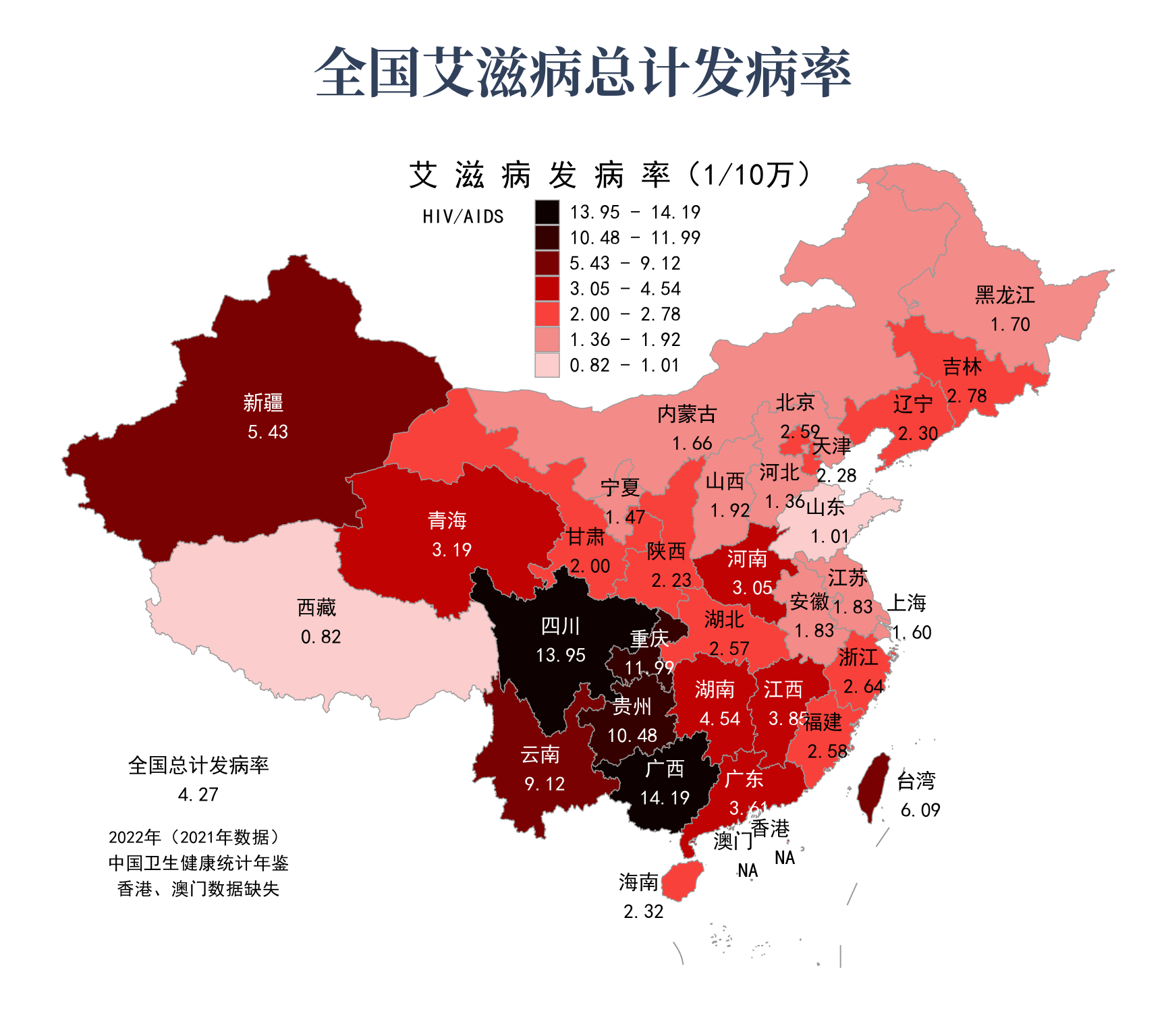
最近在小红书上看到了 2021 年中国艾滋病发病率地图,尽管有个别细节上的瑕疵,但是瑕不掩瑜,这幅图总体上比较专业,一时技痒,打算复刻这幅图。下面让我们一窥这幅图全貌:
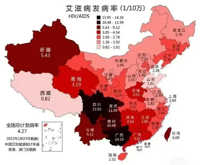
这幅图有几个亮点:
布局方面。他把南海插图放在的左下角,把图例放在内蒙古上方的外蒙古,布局很合理,而一般看到的图是把图例放在左小角,而右下角放置南海插图。
颜色方面。很醒目,从浅粉色到黑色分别映射到每个区间。注意他的区间是不连续的,这个很有意思。
标签方面。他把靠海的部分不方便在图上显示的省区放在了外面,比如海南、澳门、香港、台湾、上海、天津,用黑色标记,而其他省区是根据数值大小分成了两类,数值小于 3 的因为映射较浅的颜色,他用了黑色标签,数值大于等于 3 的因为映射较深的颜色,如果还用黑色标签就看不太清楚了,他用了白色标签。标签的位置总体是在各省区质心的基础上个别调整,例如北京、天津、甘肃、陕西和内蒙古等。
这幅图两个小小的瑕疵:
南海插图。纬度方面,曾母暗沙约 3°58′N,制图时设置 3°N 能完整包住全部南沙、曾母暗沙,而这幅图的插图紧贴着南海九段线最下边,导致地图不全。25°N 完整带出雷州半岛、两广南部海岸线,插图和主图陆地衔接视觉更自然,也是标准地图服务系统默认值;经度方面,105°E ~ 123°E 是国内论文通用标准,西抵越南河内、东抵菲律宾马尼拉,匹配规范“西面河内、东面马尼拉”的四至定义,能完整容纳九段线全部段落。而这幅宣传图的插图就显得太纠结,主图和插图衔接不自然。
缺失值问题。
NA表示数据确实存在,但我们没有收集到 / 缺失了。N/A表示数据根本不存在,或者该项指标在此处不适用。这里明显是前一种情况,应该用NA。
下面我们开始复刻这幅图。
中国地图做法
统计之都上有很多关于 R 语言画中国地图的文章和讨论。黄湘云的《R 语言画中国地图》一文中较全面介绍了中国地图的好几种做法。
首先从数据来源看,国家地理信息公共服务平台是目前最权威的数据来源,推荐使用。阿里云 DataV 数据可视化平台也提供了地图数据,它来自高德开放平台。
从地图数据处理工具看,sf 包是 R 语言现代主流矢量地理空间数据处理包,替代老旧的 sp 包,专门处理 GIS 矢量数据,底层封装三大 GIS 工业库,其中:GDAL 负责读写 shp、geojson、mdb 等地理文件,GEOS 负责平面几何运算(相交、缓冲、裁剪、质心),PROJ 负责坐标系转换、投影变换,经纬度球面运算自动调用 s2 包,精度更高。
从绘图工具来看,自然是 R 语言最著名的绘图包 ggplot2,此处不再赘述。当然了,leaflet 也是很棒的工具,值得一试。
先跑通整个工具链
从数据的可获得性、完整性和权威性三个维度看,高德平台的地图数据最容易获取,也比较完整,自带南海诸岛、钓鱼岛及其附属岛屿,无需额外添加南海诸岛和九段线图层,另外该地图数据还贴心的加入了各省区的行政中心和地理位置中心的经纬度,权威性自然与官方权威部门的数据不能比,但是这个数据有大厂背书,背后有无数的高德地图用户,还是值得信赖的,作为学习和交流使用完全没有问题,因此本次中国地图绘制使用高德平台地图数据。
# ------------------------------
# 加载 R 包
# ------------------------------

library(sf)
library(ggplot2)

# ------------------------------
# 获取数据地图
# ------------------------------

# 数据来源:https://datav.aliyun.com/portal/school/atlas/area_selector
# 数据版本:areas_v3
# 行政区划范围:中华人民共和国
# 数据粒度:省
url = "https://geo.datav.aliyun.com/areas_v3/bound/100000_full.json"

# 下载数据方便离线使用
if (!dir.exists("data")) dir.create("data")
dest = "./data/中华人民共和国省级地图数据.json"
if (!file.exists(dest)) download.file(url, dest)

# ------------------------------
# 读取地图数据
# ------------------------------

# 高德的中国行政区划 GeoJSON 是平面投影适配的矢量边界
# 禁用 s2 球面几何,使用传统 GEOS 平面笛卡尔几何
sf_use_s2(FALSE)

# 读取中国省级地图数据
cn_raw = read_sf(dest)

# ------------------------------
# 生成最终地图
# ------------------------------

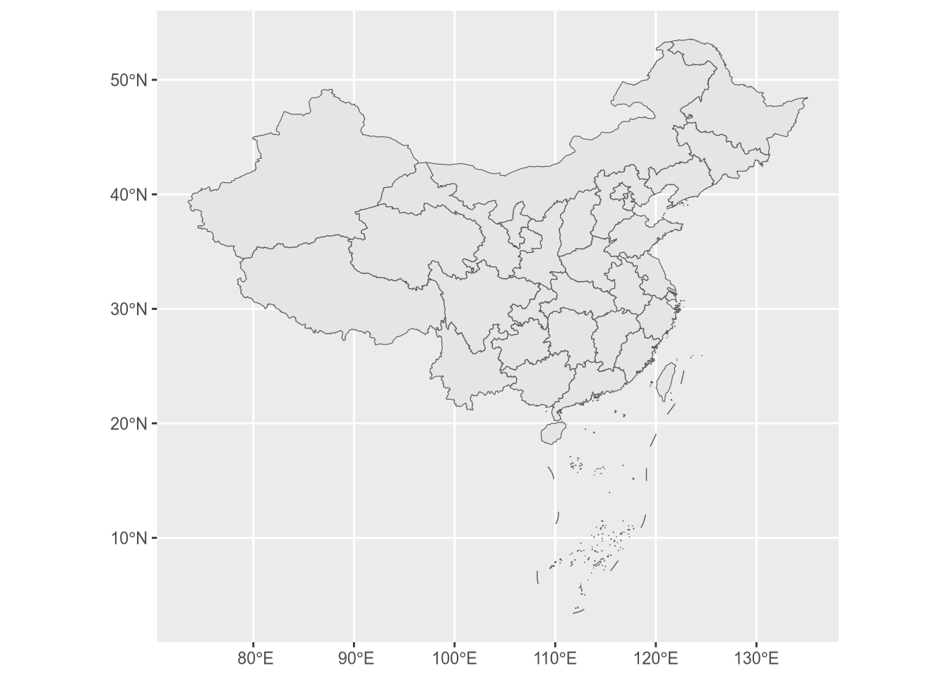
ggplot() +
  geom_sf(data = cn_raw)
实际数据映射到地图上
- 先把艾滋病发病率数据合并到地图数据里
# 加载必要的 dplyr 函数
use("dplyr", c("mutate", "select", "coalesce"))

# 艾滋病发病率数据(1/10万)
prov_aids = tibble::tribble(
  ~name,               ~value,
  "北京市",             2.59,
  "天津市",             2.28,
  "河北省",             1.36,
  "山西省",             1.92,
  "内蒙古自治区",        1.66,
  "辽宁省",             2.30,
  "吉林省",             2.78,
  "黑龙江省",           1.70,
  "上海市",             1.60,
  "江苏省",             1.83,
  "浙江省",             2.64,
  "安徽省",             1.83,
  "福建省",             2.58,
  "江西省",             3.85,
  "山东省",             1.01,
  "河南省",             3.05,
  "湖北省",             2.57,
  "湖南省",             4.54,
  "广东省",             3.61,
  "广西壮族自治区",     14.19,
  "海南省",             2.32,
  "重庆市",            11.99,
  "四川省",            13.95,
  "贵州省",            10.48,
  "云南省",             9.12,
  "西藏自治区",         0.82,
  "陕西省",             2.23,
  "甘肃省",             2.00,
  "青海省",             3.19,
  "宁夏回族自治区",      1.47,
  "新疆维吾尔自治区",    5.43,
  "台湾省",             6.09,
  "香港特别行政区",      NA,
  "澳门特别行政区",      NA
)

# 合并数据(地图数据 + 艾滋病数据)
cn_raw |>
  merge(prov_aids, by = "name", all.x = TRUE) |>
  mutate(
    interval = cut(
      value,
      breaks = c(
        0.82, 1.02, 1.36, 1.93, 2.00, 2.79, 3.05, 4.55,
        5.43, 9.13, 10.48, 12.00, 13.95, 14.20
      ),
      right = FALSE,
      labels = c(
        "0.82 - 1.01", NA, "1.36 - 1.92", NA,
        "2.00 - 2.78", NA, "3.05 - 4.54", NA,
        "5.43 - 9.12", NA, "10.48 - 11.99", NA,
        "13.95 - 14.19"
      )
    )
  ) -> cn_map
- 设置填充颜色和标签位置、内容、颜色
# 定义每个区间的颜色
interval_colors = c(
  "0.82 - 1.01"   = "#fbcdcd",  # 浅粉
  "1.36 - 1.92"   = "#f38b88",  # 深粉
  "2.00 - 2.78"   = "#f8413b",  # 红色
  "3.05 - 4.54"   = "#c00203",  # 深红
  "5.43 - 9.12"   = "#790102",  # 暗红
  "10.48 - 11.99" = "#340100",  # 黑红
  "13.95 - 14.19" = "#0d0101"   # 黑色
)

# 几何质心处标签位置微调
adjust_dict = tibble::tribble(
  ~short_name, ~lon_offset, ~lat_offset,
  "甘肃",       0.3,        -1.1,
  "内蒙古",    -4.0,        -3.5,
  "陕西",       0.0,        -1.0,
  "河北",       1.0,         0.0,
  "北京",       0.0,         1.2,
  "天津",       1.2,         0.0,
  "辽宁",       0.7,         0.0,
  "吉林",       0.0,        -0.6,
  "黑龙江",     1.0,        -1.5,
  "云南",       0.0,        -0.5,
  "海南",      -2.5,        -0.3,
  "澳门",      -0.8,        -1.8,
  "香港",       0.8,        -1.4,
  "台湾",       2.5,        -0.5,
  "上海",       1.5,         0.7
)

# 确定标签位置、内容和颜色
cn_map |>
  st_drop_geometry() |>
  subset(level == "province") |>
  mutate(
    # 根据全称生成简称
    short_name = gsub("(省|自治区|市|特别行政区)$", "", name),
    short_name = gsub("(壮族|回族|维吾尔)", "", short_name),

    # 生成标签内容并确定颜色
    label = paste(short_name, format(value, nsmall = 2), sep = "\n"),
    type = ifelse(
      # 标签在外部的一律用黑色;在内部的,数值小颜色浅用黑色,数值大颜色深用白色
      value > 3 & !short_name %in% c("海南", "澳门", "香港", "台湾", "上海", "天津"),
      "white_font", "black_font"
    ),

    # 提取省区行政中心和质心
    c_lon = vapply(center, `[`, numeric(1), 1),
    c_lat = vapply(center, `[`, numeric(1), 2),
    geo_lon = vapply(centroid, `[`, numeric(1), 1),
    geo_lat = vapply(centroid, `[`, numeric(1), 2),

    # 河北、甘肃几何质心缺失,先用行政中心补齐
    geo_lon = ifelse(short_name %in% c("河北", "甘肃"), c_lon, geo_lon),
    geo_lat = ifelse(short_name %in% c("河北", "甘肃"), c_lat, geo_lat)
  ) |>
  select(short_name, label, type, interval, geo_lon, geo_lat) |>

  # 匹配标签位置微调参数并调整
  merge(adjust_dict, by = "short_name", all.x = TRUE) |>
  mutate(
    geo_lon = geo_lon + coalesce(lon_offset, 0),
    geo_lat = geo_lat + coalesce(lat_offset, 0)
  ) |>
  select(
    -lon_offset, -lat_offset
  ) -> prov_labels
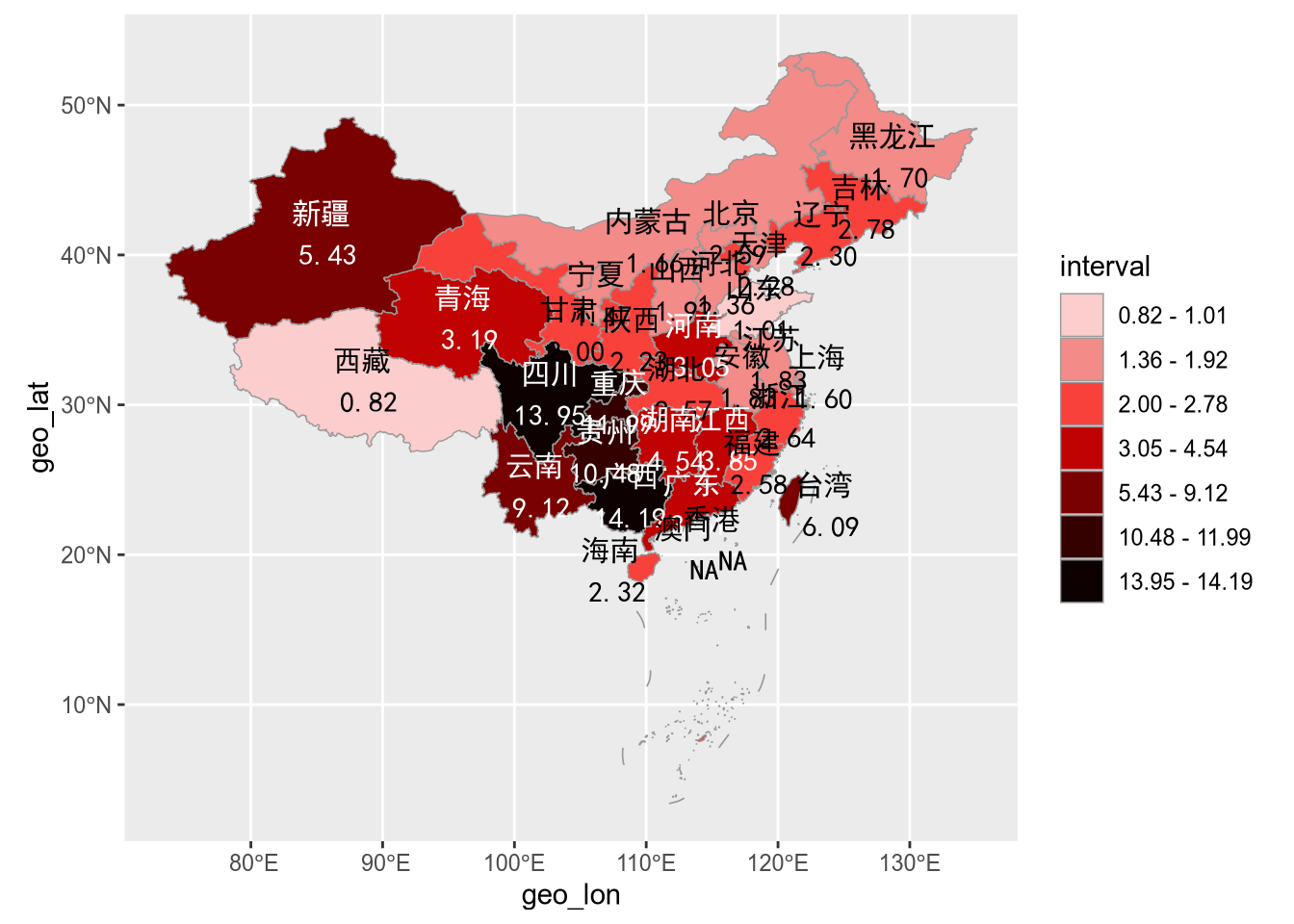
- 生成省区填充色映射艾滋病数据的地图
ggplot() +
  # 绘制中国地图最底层图层
  geom_sf(
    data = cn_map, aes(fill = interval),
    color = "gray60", linewidth = 0.25
  ) +

  # 标注各省区简称和艾滋病发病率
  geom_text(
    data = prov_labels,
    aes(x = geo_lon, y = geo_lat, label = label, color = type),
    size = 4, family = "SimHei", hjust = 0.5
  ) +
  scale_color_manual(
    values = c("black_font" = "black", "white_font" = "white"),
    guide = "none"
  ) +

  # 各省区艾滋病发病率数值按区间填充颜色
  scale_fill_manual(
    values = interval_colors,
    na.value = "white",    # 缺失值省区填充白色
    na.translate = FALSE,  # 隐藏缺失值图例
  ) -> p1

print(p1)
再出发,美化地图
完成了上面的图,剩下的工作除了南海九段线插图外,都没什么技术含量,但是参数调整比较耗费时间。我们先修改图例位置和顺序、加入注释说明、砍掉涂上艾滋病发病率信息密度极低的下半部分、调整图片尺寸。
p1 +
  # 设置地图标题、图例、范围和坐标系
  labs(title = "全国艾滋病总计发病率") +
  guides(fill = guide_legend(reverse = TRUE, title = NULL)) +
  coord_sf(xlim = c(73, 136), ylim = c(16, 54), expand = FALSE) +

  # 正上方添加图例注解
  annotate(
    "text", x = 106, y = 52,
    label = "艾 滋 病 发 病 率(1/10万)",
    family = "SimHei", size = 6
  ) +
  annotate(
    "text", x = 98.5, y = 50.5,
    label = "HIV/AIDS",
    family = "SimHei", size = 4
  ) +

  # 左小角添加注解说明
  annotate(
    "text", x = 82.5, y = 24,
    label = "全国总计发病率\n4.27",
    family = "SimHei", size = 5
  ) +
  annotate(
    "text", x = 82.5, y = 20,
    label = "2022年(2021年数据)\n中国卫生健康统计年鉴\n香港、澳门数据缺失",
    family = "SimHei", size = 4
  ) +

  # 设置地图主题
  theme_void() +
  theme(
    plot.title = element_text(
      family = "Noto Serif CJK SC", color = "#31415b",
      size = 30, face = "bold", hjust = 0.5, vjust = 1.5
    ),
    legend.background = element_blank(),
    legend.position = c(0.53, 0.82),
    legend.key.size = unit(0.50, "cm"),
    legend.text = element_text(family = "SimHei", size = 11)
  ) -> p2

print(p2)
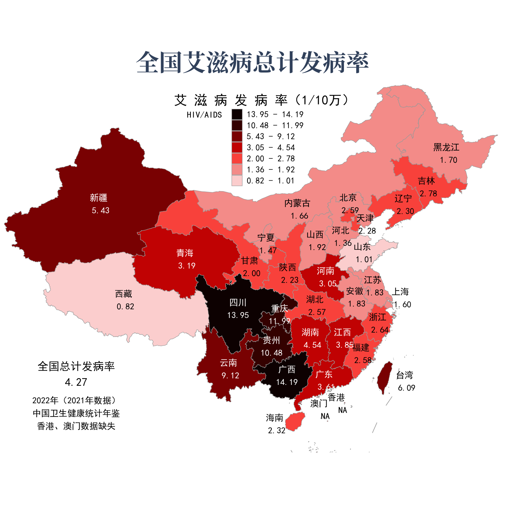
注意:为了追求视觉效果,南海下半部分被砍了,但是必须保证地图完整,这就需要在地图上加一个插图专门显示南海岛礁和九段线等。
添加南海九段线插图
- 南海插图参数设置和矢量坐标转换
# 能囊括完整南海四至的范围(包含全部岛礁、九段线)
nh_lon_min = 105
nh_lon_max = 123
nh_lat_min = 3
nh_lat_max = 25

# 确定插图画布尺寸
nh_w = nh_lon_max - nh_lon_min  # 经度宽度
nh_h = nh_lat_max - nh_lat_min  # 纬度高度
nh_aspect_ratio = nh_h / nh_w

inset_w = 7
inset_h = inset_w * nh_aspect_ratio

# 插图放置起点(经纬度坐标)
inset_x0 = 88.5
inset_y0 = 17

# 生成南海插图地图数据
clip_bbox = st_bbox(
  c(
    xmin = nh_lon_min, ymin = nh_lat_min,
    xmax = nh_lon_max, ymax = nh_lat_max
  ),
  crs = 4326
)

scale_matrix = matrix(
  c(
    inset_w / (nh_lon_max - nh_lon_min), 0,
    0, inset_h / (nh_lat_max - nh_lat_min)
  ),
  ncol = 2
)

cn_map |>
  st_make_valid() |>
  st_crop(clip_bbox) |>
  mutate(
    geometry = (geometry - c(nh_lon_min, nh_lat_min)) *
      scale_matrix + c(inset_x0, inset_y0)
  ) |>
  st_set_geometry("geometry") |>
  st_set_crs(4326) -> nh_inset
- 生成完整的艾滋病发病率可视化地图
p2 +
  # 绘制南海插图背景
  geom_rect(
    aes(
      xmin = inset_x0, xmax = inset_x0 + inset_w,
      ymin = inset_y0, ymax = inset_y0 + inset_h
    ),
    fill = "white", color = "black", linewidth = 0.25
  ) +

  # 插图内绘制南海诸岛
  geom_sf(
    data = nh_inset,
    aes(fill = interval),
    color = "gray60", linewidth = 0.25
  ) +

  # 设置主图显示范围
  coord_sf(
    xlim = c(73, 136), ylim = c(16, 54), expand = FALSE
  ) -> p3

print(p3)
附上完整代码方便重现
#'
#' 科学绘制中国地图(WGS84)
#'
#' @author 楚新元
#' @date 2026-06-20
#'

# ------------------------------
# 加载 R 包
# ------------------------------

library(sf)
library(ggplot2)
use("dplyr", c("mutate", "select", "coalesce"))

# ------------------------------
# 获取数据地图
# ------------------------------

# 数据来源:https://datav.aliyun.com/portal/school/atlas/area_selector
# 数据版本:areas_v3
# 行政区划范围:中华人民共和国
# 数据粒度:省
url = "https://geo.datav.aliyun.com/areas_v3/bound/100000_full.json"

# 下载数据方便离线使用
if (!dir.exists("data")) dir.create("data")
dest = "./data/中华人民共和国省级地图数据.json"
if (!file.exists(dest)) download.file(url, dest)

# ------------------------------
# 地图数据和艾滋病数据并合并
# ------------------------------

# 高德的中国行政区划 GeoJSON 是平面投影适配的矢量边界
# 禁用 s2 球面几何,使用传统 GEOS 平面笛卡尔几何
sf_use_s2(FALSE)

# 读取中国省级地图数据
cn_raw = read_sf(dest)

# 艾滋病发病率数据(1/10万)
prov_aids = tibble::tribble(
  ~name,               ~value,
  "北京市",             2.59,
  "天津市",             2.28,
  "河北省",             1.36,
  "山西省",             1.92,
  "内蒙古自治区",        1.66,
  "辽宁省",             2.30,
  "吉林省",             2.78,
  "黑龙江省",           1.70,
  "上海市",             1.60,
  "江苏省",             1.83,
  "浙江省",             2.64,
  "安徽省",             1.83,
  "福建省",             2.58,
  "江西省",             3.85,
  "山东省",             1.01,
  "河南省",             3.05,
  "湖北省",             2.57,
  "湖南省",             4.54,
  "广东省",             3.61,
  "广西壮族自治区",     14.19,
  "海南省",             2.32,
  "重庆市",            11.99,
  "四川省",            13.95,
  "贵州省",            10.48,
  "云南省",             9.12,
  "西藏自治区",         0.82,
  "陕西省",             2.23,
  "甘肃省",             2.00,
  "青海省",             3.19,
  "宁夏回族自治区",      1.47,
  "新疆维吾尔自治区",    5.43,
  "台湾省",             6.09,
  "香港特别行政区",      NA,
  "澳门特别行政区",      NA
)

# 合并数据(地图数据 + 艾滋病数据)
cn_raw |>
  merge(prov_aids, by = "name", all.x = TRUE) |>
  mutate(
    interval = cut(
      value,
      breaks = c(
        0.82, 1.02, 1.36, 1.93, 2.00, 2.79, 3.05, 4.55,
        5.43, 9.13, 10.48, 12.00, 13.95, 14.20
      ),
      right = FALSE,
      labels = c(
        "0.82 - 1.01", NA, "1.36 - 1.92", NA,
        "2.00 - 2.78", NA, "3.05 - 4.54", NA,
        "5.43 - 9.12", NA, "10.48 - 11.99", NA,
        "13.95 - 14.19"
      )
    )
  ) -> cn_map

# ------------------------------
# 设置填充颜色和标签位置、内容、颜色
# ------------------------------

# 定义每个区间的颜色
interval_colors = c(
  "0.82 - 1.01"   = "#fbcdcd",  # 浅粉
  "1.36 - 1.92"   = "#f38b88",  # 深粉
  "2.00 - 2.78"   = "#f8413b",  # 红色
  "3.05 - 4.54"   = "#c00203",  # 深红
  "5.43 - 9.12"   = "#790102",  # 暗红
  "10.48 - 11.99" = "#340100",  # 黑红
  "13.95 - 14.19" = "#0d0101"   # 黑色
)

# 几何质心处标签位置微调
adjust_dict = tibble::tribble(
  ~short_name, ~lon_offset, ~lat_offset,
  "甘肃",       0.3,        -1.1,
  "内蒙古",    -4.0,        -3.5,
  "陕西",       0.0,        -1.0,
  "河北",       1.0,         0.0,
  "北京",       0.0,         1.2,
  "天津",       1.2,         0.0,
  "辽宁",       0.7,         0.0,
  "吉林",       0.0,        -0.6,
  "黑龙江",     1.0,        -1.5,
  "云南",       0.0,        -0.5,
  "海南",      -2.5,        -0.3,
  "澳门",      -0.8,        -1.8,
  "香港",       0.8,        -1.4,
  "台湾",       2.5,        -0.5,
  "上海",       1.5,         0.7
)

# 确定标签位置、内容和颜色
cn_map |>
  st_drop_geometry() |>
  subset(level == "province") |>
  mutate(
    # 根据全称生成简称
    short_name = gsub("(省|自治区|市|特别行政区)$", "", name),
    short_name = gsub("(壮族|回族|维吾尔)", "", short_name),

    # 生成标签内容并确定颜色
    label = paste(short_name, format(value, nsmall = 2), sep = "\n"),
    type = ifelse(
      # 标签在外部的一律用黑色;在内部的,数值小颜色浅用黑色,数值大颜色深用白色
      value > 3 & !short_name %in% c("海南", "澳门", "香港", "台湾", "上海", "天津"),
      "white_font", "black_font"
    ),

    # 提取省区行政中心和质心
    c_lon = vapply(center, `[`, numeric(1), 1),
    c_lat = vapply(center, `[`, numeric(1), 2),
    geo_lon = vapply(centroid, `[`, numeric(1), 1),
    geo_lat = vapply(centroid, `[`, numeric(1), 2),

    # 河北、甘肃几何质心缺失,先用行政中心补齐
    geo_lon = ifelse(short_name %in% c("河北", "甘肃"), c_lon, geo_lon),
    geo_lat = ifelse(short_name %in% c("河北", "甘肃"), c_lat, geo_lat)
  ) |>
  select(short_name, label, type, interval, geo_lon, geo_lat) |>

  # 匹配标签位置微调参数并调整
  merge(adjust_dict, by = "short_name", all.x = TRUE) |>
  mutate(
    geo_lon = geo_lon + coalesce(lon_offset, 0),
    geo_lat = geo_lat + coalesce(lat_offset, 0)
  ) |>
  select(
    -lon_offset, -lat_offset
  ) -> prov_labels

# ------------------------------
# 南海插图参数设置和矢量坐标转换
# ------------------------------

# 能囊括完整南海四至的范围(包含全部岛礁、九段线)
nh_lon_min = 105
nh_lon_max = 123
nh_lat_min = 3
nh_lat_max = 25

# 确定插图画布尺寸
nh_w = nh_lon_max - nh_lon_min  # 经度宽度
nh_h = nh_lat_max - nh_lat_min  # 纬度高度
nh_aspect_ratio = nh_h / nh_w

inset_w = 7
inset_h = inset_w * nh_aspect_ratio

# 插图放置起点(经纬度坐标)
inset_x0 = 88.5
inset_y0 = 17

# 生成南海插图地图数据
clip_bbox = st_bbox(
  c(
    xmin = nh_lon_min, ymin = nh_lat_min,
    xmax = nh_lon_max, ymax = nh_lat_max
  ),
  crs = 4326
)

scale_matrix = matrix(
  c(
    inset_w / (nh_lon_max - nh_lon_min), 0,
    0, inset_h / (nh_lat_max - nh_lat_min)
  ),
  ncol = 2
)

cn_map |>
  st_make_valid() |>
  st_crop(clip_bbox) |>
  mutate(
    geometry = (geometry - c(nh_lon_min, nh_lat_min)) *
      scale_matrix + c(inset_x0, inset_y0)
  ) |>
  st_set_geometry("geometry") |>
  st_set_crs(4326) -> nh_inset

# ------------------------------
# 生成最终地图
# ------------------------------

ggplot() +
  # 绘制中国地图最底层图层
  geom_sf(
    data = cn_map, aes(fill = interval),
    color = "gray60", linewidth = 0.25
  ) +

  # 绘制南海插图背景
  geom_rect(
    aes(
      xmin = inset_x0, xmax = inset_x0 + inset_w,
      ymin = inset_y0, ymax = inset_y0 + inset_h
    ),
    fill = "white", color = "black", linewidth = 0.25
  ) +

  # 插图内绘制南海诸岛
  geom_sf(
    data = nh_inset, aes(fill = interval),
    color = "gray60", linewidth = 0.25
  ) +

  # 标注各省区简称和艾滋病发病率
  geom_text(
    data = prov_labels,
    aes(x = geo_lon, y = geo_lat, label = label, color = type),
    size = 4, family = "SimHei", hjust = 0.5
  ) +
  scale_color_manual(
    values = c("black_font" = "black", "white_font" = "white"),
    guide = "none"
  ) +

  # 各省区艾滋病发病率数值按区间填充颜色
  scale_fill_manual(
    values = interval_colors,
    na.value = "white",    # 缺失值省区填充白色
    na.translate = FALSE,  # 隐藏缺失值图例
  ) +

  # 设置地图标题、图例、范围和坐标系
  labs(title = "全国艾滋病总计发病率") +
  guides(fill = guide_legend(reverse = TRUE, title = NULL)) +
  coord_sf(xlim = c(73, 136), ylim = c(16, 54), expand = FALSE) +

  # 正上方添加图例注解
  annotate(
    "text", x = 106, y = 52,
    label = "艾 滋 病 发 病 率(1/10万)",
    family = "SimHei", size = 6
  ) +
  annotate(
    "text", x = 98.5, y = 50.5,
    label = "HIV/AIDS",
    family = "SimHei", size = 4
  ) +

  # 左小角添加注解说明
  annotate(
    "text", x = 82.5, y = 24,
    label = "全国总计发病率\n4.27",
    family = "SimHei", size = 5
  ) +
  annotate(
    "text", x = 82.5, y = 20,
    label = "2022年(2021年数据)\n中国卫生健康统计年鉴\n香港、澳门数据缺失",
    family = "SimHei", size = 4
  ) +

  # 设置地图主题
  theme_void() +
  theme(
    plot.title = element_text(
      family = "Noto Serif CJK SC", color = "#31415b",
      size = 30, face = "bold", hjust = 0.5, vjust = 1.5
    ),
    legend.background = element_blank(),
    legend.position = c(0.53, 0.82),
    legend.key.size = unit(0.50, "cm"),
    legend.text = element_text(family = "SimHei", size = 11)
  )
- 注意 2026-06-21
上面的代码生成的图作为日常学习交流使用完全没问题,但是在学术论文和正式场合,建议还是使用官方权威数据来源,如国家地理信息公共服务平台;另外,本文生成的地图和国内权威媒体通常使用的地图形状有些差异,我们的图看起来比较扁,这其实是因为基础坐标系和投影不同而造成的,我们使用的是默认的 WGS84 坐标系,而权威媒体的地图坐标系采用 2000 国家大地坐标系(CGCS2000),投影方式选用 Albers 等面积圆锥投影(基准面:CGCS2000),中央经线 105°E,标准纬线 25°N、47°N。
环境信息
xfun::session_info()
#> R version 4.6.0 (2026-04-24)
#> Platform: x86_64-pc-linux-gnu
#> Running under: Arch Linux, Positron 2026.06.0
#>
#> Locale:
#>   LC_CTYPE=en_US.UTF-8       LC_NUMERIC=C
#>   LC_TIME=zh_CN.UTF-8        LC_COLLATE=en_US.UTF-8
#>   LC_MONETARY=zh_CN.UTF-8    LC_MESSAGES=en_US.UTF-8
#>   LC_PAPER=zh_CN.UTF-8       LC_NAME=C
#>   LC_ADDRESS=C               LC_TELEPHONE=C
#>   LC_MEASUREMENT=zh_CN.UTF-8 LC_IDENTIFICATION=C
#>
#> Package version:
#>   base64enc_0.1.6    blogdown_1.24      bookdown_0.47      bslib_0.11.0
#>   cachem_1.1.0       class_7.3-23       classInt_0.4-11    cli_3.6.6
#>   compiler_4.6.0     cpp11_0.5.5        DBI_1.3.0          digest_0.6.39
#>   dplyr_1.2.1        e1071_1.7-17       evaluate_1.0.5     farver_2.1.2
#>   fastmap_1.2.0      fontawesome_0.5.3  fs_2.1.0           generics_0.1.4
#>   ggplot2_4.0.3      glue_1.8.1         graphics_4.6.0     grDevices_4.6.0
#>   grid_4.6.0         gtable_0.3.6       highr_0.12         htmltools_0.5.9
#>   httpuv_1.6.17      isoband_0.3.0      jpeg_0.1-11        jquerylib_0.1.4
#>   jsonlite_2.0.0     KernSmooth_2.23-26 knitr_1.51         labeling_0.4.3
#>   later_1.4.8        lifecycle_1.0.5    magrittr_2.0.5     MASS_7.3.65
#>   memoise_2.0.1      methods_4.6.0      mime_0.13          otel_0.2.0
#>   pillar_1.11.1      pkgconfig_2.0.3    promises_1.5.0     proxy_0.4-29
#>   R6_2.6.1           rappdirs_0.3.4     RColorBrewer_1.1-3 Rcpp_1.1.1-1.1
#>   rlang_1.2.0        rmarkdown_2.31     s2_1.1.11          S7_0.2.2
#>   sass_0.4.10        scales_1.4.0       servr_0.33         sf_1.1-1
#>   stats_4.6.0        tibble_3.3.1       tidyselect_1.2.1   tinytex_0.60
#>   tools_4.6.0        units_1.0-1        utf8_1.2.6         utils_4.6.0
#>   vctrs_0.7.3        viridisLite_0.4.3  withr_3.0.3        wk_0.9.5
#>   xfun_0.59          yaml_2.3.12