
主成分分析
楚新元 / 2025-07-04
本文是《精通机器学习:基于 R》(第 2 版)学习笔记。不清楚的地方请读者翻看原文。
理解主成分分析
信息过度复杂是多变量数据最大的挑战之一。若数据集有 100 个变量,如何了解其中所有的交互关系呢?即使只有 20 个变量,当试图理解各个变量与其他变量的关系时,也需要考虑 190 对 相互关系。主成分分析(PCA)是一种数据降维技巧,它能将大量相关变量转化为一组很少的不相关变量,这些无关变量称为主成分,并且尽可能地保留原始数据集的信息。
对于主成分模型构建过程,模型构建与评价步骤,我们按照以下几个步骤进行:
抽取主成分并决定保留的数量;
对留下的主成分进行旋转;
对旋转后的解决方案进行解释;
生成各个因子的得分;
使用得分作为输入变量进行回归分析,并使用测试数据评价模型效果。
下面是一个主成分分析实战案例,进一步学习该模型的应用。
数据准备
library(ggplot2)
library(psych)
train = read.csv("./data/NHLtrain.csv")
head(train)
#>       Team  ppg Goals_For Goals_Against Shots_For Shots_Against PP_perc PK_perc
#> 1  Anaheim 1.26      2.62          2.29      30.3          27.5    23.0    87.2
#> 2  Arizona 0.95      2.54          2.98      27.6          31.0    17.7    77.3
#> 3   Boston 1.13      2.88          2.78      32.0          30.4    20.5    82.2
#> 4  Buffalo 0.99      2.43          2.62      29.5          30.6    18.9    82.6
#> 5  Calgary 0.94      2.79          3.13      29.2          29.0    17.0    75.6
#> 6 Carolina 1.05      2.39          2.70      29.9          27.6    16.8    84.3
#>   CF60_pp CA60_sh OZFOperc_pp Give Take  hits  blks
#> 1  111.64   94.07     78.4141 9.78 5.22 27.24 14.37
#> 2   97.65   96.06     72.5217 5.67 5.89 22.13 14.02
#> 3  118.33   94.43     79.4393 8.60 6.11 26.39 14.44
#> 4   97.39  100.57     76.2105 6.34 5.26 23.37 13.35
#> 5   94.00  102.79     77.0624 9.80 6.99 20.73 16.10
#> 6  102.95   80.65     81.3953 8.00 9.22 18.90 11.95
这个数据集包含 30 支大联盟球队的统计数据1,目标是建立一个模型来预测一支队伍的总积分,通过 PCA 建立一个输入特征空间,目的是揭示哪些因素能够造就一支顶级职业球队。其中各字段的含义如下:
- Team:球队所在城市。
- ppg:平均每场得分。
- Goals_For:平均每场进球数。
- Goals_Against:平均每场失球数。
- Shots_For:平均每场射中球门次数。
- Shots_Against:平均每场被射中球门次数。
- PP_perc:球队以多打少时进球百分比。
- PK_perc:球队以多打少球门不失的时间百分比。
- CF60_pp:球队在每 60 分钟以多打少时间内获得的 Corsi 分值;Corsi 分值是射门次数总和。
- CA60_sh:对手在每 60 分钟以多打少时间内获得的 Corsi 分值。
- OZFOperc_pp:球队以多打少时,在进攻区域发生的争球次数百分比。
- Give:平均每场的丢球次数。
- Take:平均每场抢断次数。
- hits:平均每场身体冲撞次数。
- blks:平均每场封堵对方射门次数。
探索性数据分析
首先对数据进行标准化处理,使数据的均值为 0,标准差为 1。完成标准化后,创建一个输入特征的相关性统计图。
library(corrplot)
train_scale = scale(train[, -1:-2])
train_scale_m = cor(train_scale)
corrplot(
  train_scale_m,
  type = "lower",
  order = "hclust",
  col = c("black", "red"),
  bg = "white"
)
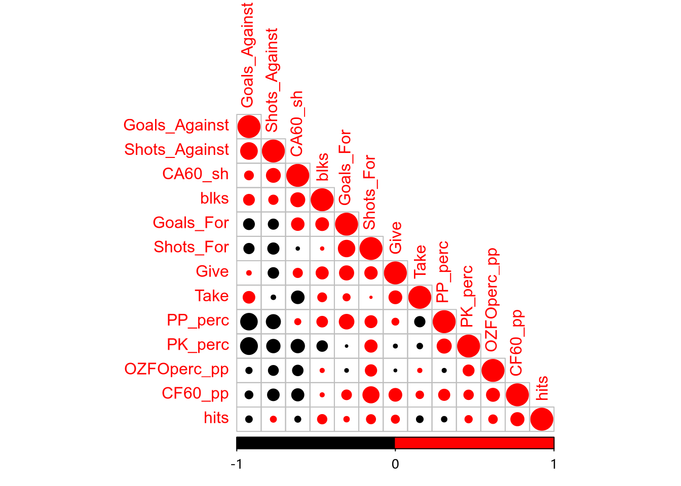
从相关系数图上可以看出,Shots_For 和 Goals_For 正相关,Shots_Against 和 Goals_Against 正相关,PP_perc 及 PK_perc 与 Goals_Against 负相关。由此可知,这个数据集非常适合提取主成分。
判断主成分个数
fa.parallel(
  train_scale,
  fa = "pc",
  n.iter = 100,
  show.legend = FALSE,
  main = "Scree plot with parallel analysis"
)
#> Parallel analysis suggests that the number of factors = NA and the number of components = 3
abline(h = 1, lwd = 0.8, col = "green")
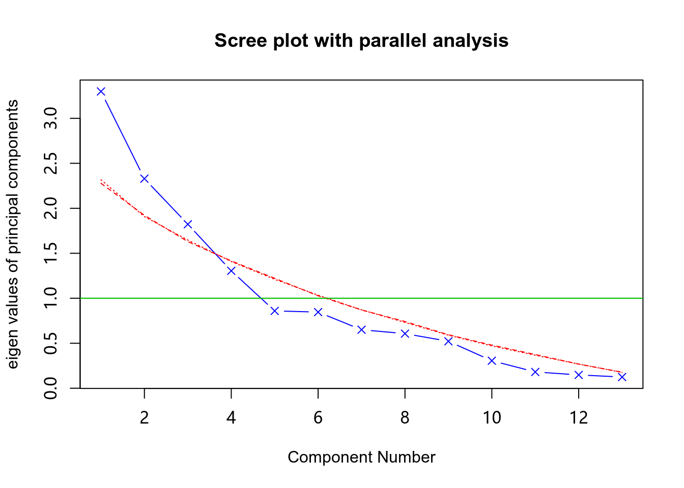
上图展示了基于观测值特征值的碎石检验,根据 100 个随机数据矩阵推导出来的特征值均线(虚线),以及大于 1 的特征值准则表明保留 4 个主成分即可,5 个主成分是很令人信服的。
经验表明:主成分解释的方差累加起来,应该能够解释 70% 的方差。
正交旋转与解释
pca_rotate = principal(
  train_scale,
  nfactors = 5,
  rotate = "varimax"
)
print(pca_rotate)
#> Principal Components Analysis
#> Call: principal(r = train_scale, nfactors = 5, rotate = "varimax")
#> Standardized loadings (pattern matrix) based upon correlation matrix
#>                 RC1   RC2   RC5   RC3   RC4   h2   u2 com
#> Goals_For     -0.21  0.82  0.21  0.05 -0.11 0.78 0.22 1.3
#> Goals_Against  0.88 -0.02 -0.05  0.21  0.00 0.82 0.18 1.1
#> Shots_For     -0.22  0.43  0.76 -0.02 -0.10 0.81 0.19 1.8
#> Shots_Against  0.73 -0.02 -0.20 -0.29  0.20 0.70 0.30 1.7
#> PP_perc       -0.73  0.46 -0.04 -0.15  0.04 0.77 0.23 1.8
#> PK_perc       -0.73 -0.21  0.22 -0.03  0.10 0.64 0.36 1.4
#> CF60_pp       -0.20  0.12  0.71  0.24  0.29 0.69 0.31 1.9
#> CA60_sh        0.35  0.66 -0.25 -0.48 -0.03 0.85 0.15 2.8
#> OZFOperc_pp   -0.02 -0.18  0.70 -0.01  0.11 0.53 0.47 1.2
#> Give          -0.02  0.58  0.17  0.52  0.10 0.65 0.35 2.2
#> Take           0.16  0.02  0.01  0.90 -0.05 0.83 0.17 1.1
#> hits          -0.02 -0.01  0.27 -0.06  0.87 0.83 0.17 1.2
#> blks           0.19  0.63 -0.18  0.14  0.47 0.70 0.30 2.4
#>
#>                        RC1  RC2  RC5  RC3  RC4
#> SS loadings           2.69 2.33 1.89 1.55 1.16
#> Proportion Var        0.21 0.18 0.15 0.12 0.09
#> Cumulative Var        0.21 0.39 0.53 0.65 0.74
#> Proportion Explained  0.28 0.24 0.20 0.16 0.12
#> Cumulative Proportion 0.28 0.52 0.72 0.88 1.00
#>
#> Mean item complexity =  1.7
#> Test of the hypothesis that 5 components are sufficient.
#>
#> The root mean square of the residuals (RMSR) is  0.08
#>  with the empirical chi square  28.59  with prob <  0.19
#>
#> Fit based upon off diagonal values = 0.91
- SS loadings 行包含了与主成分相关联的特征值。
- Proportion Var 行表示的是每个主成分对整个数据集的解释程度。
- Cumulative Var 行表示的是主成分对整个数据集的累计解释程度。
- Proportion Explained 表示解释贡献度占比。
- Cumulative Proportion 表示解释累计贡献度。
对于第一个主成分,变量 Goals_Against 和 Shots_Against 具有非常高的正载荷,而 PP_perc 和 PK_perc 具有非常高的负载荷。
第一个主成分解释了 21% 的方差, 第二个主成分解释了 18% 的方差,……,五个主成分累计解释了 74% 的方差。
根据主成分建立因子得分
round(unclass(pca_rotate$weights), 2)
#>                 RC1   RC2   RC5   RC3   RC4
#> Goals_For     -0.02  0.36  0.10 -0.01 -0.18
#> Goals_Against  0.36  0.01  0.12  0.10 -0.06
#> Shots_For      0.09  0.17  0.49 -0.14 -0.26
#> Shots_Against  0.28  0.00  0.03 -0.21  0.15
#> PP_perc       -0.32  0.19 -0.18 -0.06  0.08
#> PK_perc       -0.29 -0.12 -0.01  0.00  0.13
#> CF60_pp        0.03  0.01  0.34  0.07  0.15
#> CA60_sh        0.15  0.31 -0.03 -0.33 -0.07
#> OZFOperc_pp    0.13 -0.10  0.46 -0.12 -0.02
#> Give           0.00  0.23 -0.01  0.32  0.04
#> Take           0.02  0.00 -0.10  0.60 -0.03
#> hits          -0.03 -0.07  0.01 -0.05  0.76
#> blks           0.00  0.25 -0.22  0.12  0.42
利用如下公式可得到主成分得分:
RC1 = -0.02 * Goals_For + 0.36 * Goals_Against + …… + 0.00 * blks
需要注意的是注意:这里的 Goals_For 等变量是 train_scale 数据中的变量,即标准化之后的变量。这里我们就不手动计算了,直接用代码生成结果:
pca_scores = data.frame(pca_rotate$scores)
head(pca_scores)
#>           RC1          RC2        RC5        RC3        RC4
#> 1 -2.21526408  0.002821488  0.3161588 -0.1572320  1.5278033
#> 2  0.88147630 -0.569239044 -1.2361419 -0.2703150 -0.0113224
#> 3  0.10321189  0.481754024  1.8135052 -0.1606672  0.7346531
#> 4 -0.06630166 -0.630676083 -0.2121434 -1.3086231  0.1541255
#> 5  1.49662977  1.156905747 -0.3222194  0.9647145 -0.6564827
#> 6 -0.48902169 -2.119952370  1.0456190  2.7375097 -1.3735777
回归分析
# 将响应变量作为一列加入数据
pca_scores$ppg = train$ppg

# 建立多元线性回归模型
fit1 = lm(ppg ~ ., data = pca_scores)
summary(fit1)
#>
#> Call:
#> lm(formula = ppg ~ ., data = pca_scores)
#>
#> Residuals:
#>       Min        1Q    Median        3Q       Max
#> -0.163274 -0.048189  0.003718  0.038723  0.165905
#>
#> Coefficients:
#>              Estimate Std. Error t value Pr(>|t|)
#> (Intercept)  1.111333   0.015752  70.551  < 2e-16 ***
#> RC1         -0.112201   0.016022  -7.003 3.06e-07 ***
#> RC2          0.070991   0.016022   4.431 0.000177 ***
#> RC5          0.022945   0.016022   1.432 0.164996
#> RC3         -0.017782   0.016022  -1.110 0.278044
#> RC4         -0.005314   0.016022  -0.332 0.743003
#> ---
#> Signif. codes:  0 '***' 0.001 '**' 0.01 '*' 0.05 '.' 0.1 ' ' 1
#>
#> Residual standard error: 0.08628 on 24 degrees of freedom
#> Multiple R-squared:  0.7502,	Adjusted R-squared:  0.6981
#> F-statistic: 14.41 on 5 and 24 DF,  p-value: 1.446e-06
回归结果表明,模型在整体上是显著的,修正后的拟合优度接近 0.7,但是有 3 个主成分是不显著的,可以简单处理,选择保留,但是我们不妨只保留 RC1 和 RC2 看看结果如何:
fit2 = lm(ppg ~ RC1 + RC2, data = pca_scores)
summary(fit2)
#>
#> Call:
#> lm(formula = ppg ~ RC1 + RC2, data = pca_scores)
#>
#> Residuals:
#>      Min       1Q   Median       3Q      Max
#> -0.18914 -0.04430  0.01438  0.05645  0.16469
#>
#> Coefficients:
#>             Estimate Std. Error t value Pr(>|t|)
#> (Intercept)  1.11133    0.01587  70.043  < 2e-16 ***
#> RC1         -0.11220    0.01614  -6.953  1.8e-07 ***
#> RC2          0.07099    0.01614   4.399 0.000153 ***
#> ---
#> Signif. codes:  0 '***' 0.001 '**' 0.01 '*' 0.05 '.' 0.1 ' ' 1
#>
#> Residual standard error: 0.0869 on 27 degrees of freedom
#> Multiple R-squared:  0.7149,	Adjusted R-squared:  0.6937
#> F-statistic: 33.85 on 2 and 27 DF,  p-value: 4.397e-08
模型 2 拟合优度几乎没有多大变化,但是模型更简练。因此我们选择模型 2(我们可以用其他准则来选择模型,结果也是模型 2 比模型 1 更优)。
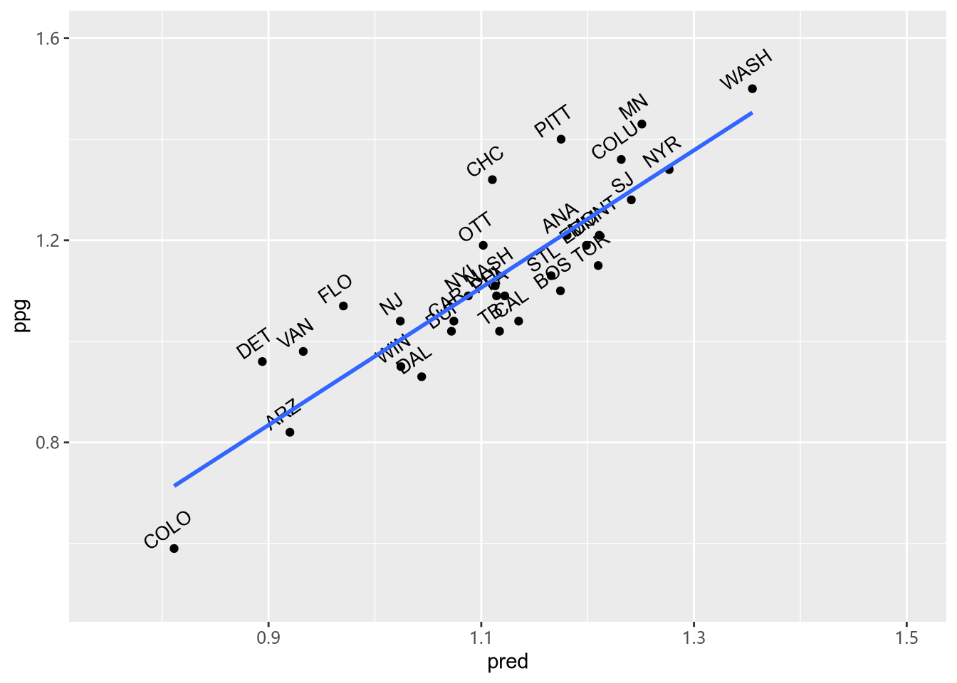
train$pred = round(fit2$fitted.values, 2)
ggplot(train, aes(pred, ppg, label = Team)) +
  geom_point() +
  geom_text(size = 3.5, hjust = 0.1, vjust = -0.5, angle = 0) +
  xlim(0.8,1.4) +  ylim(0.8, 1.5) +
  geom_smooth(method = "lm", se = FALSE)
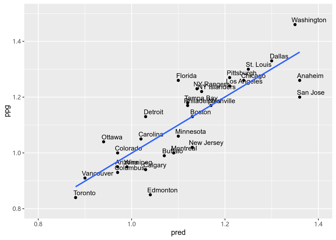
从上图我们可以看出,主成分和球队积分之间存在强烈的线性关系。
另一项分析内容是绘制出球队及其因子得分之间的关系。
pca_scores$Team = train$Team
ggplot(pca_scores, aes(RC1, RC2, label = Team)) +
  geom_point() +
  geom_text(size = 2.75, hjust = 0.2, vjust = -0.75, angle = 0)+
  xlim(-2.5, 2.5) + ylim(-3.0, 2.5)
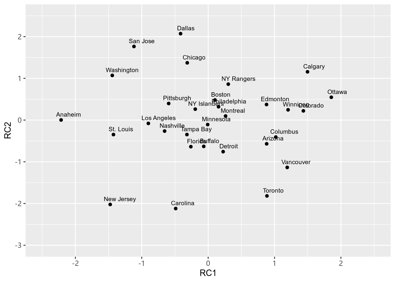
我们以 Anaheim 为对象进行简单分析,我们发现这个队 RC1 比较低,RC2 处在中间位置,RC1 上,PP_perc 和 PK_perc 具有负载荷,Goals_Against 具有正载荷,说明这只球队防守组织的比较好。
模型的均方根误差:
sqrt(mean(fit2$residuals^2))
#> [1] 0.08244449
模型预测效果评价
test = read.csv("./data/NHLtest.csv")
test_scores = data.frame(predict(
  pca_rotate,
  scale(test[, c(-1:-2)])
))
test_scores$pred = predict(fit2, test_scores)
test_scores$ppg = test$ppg
test_scores$Team = test$Team

ggplot(test_scores, aes(pred, ppg, label = Team)) +
  geom_point() +
  geom_text(size = 3.5, hjust = 0.4, vjust = -0.9, angle = 35)+
  xlim(0.75, 1.5) + ylim(0.5, 1.6) +
  geom_smooth(method = "lm", se = FALSE)
最后,再检查以下 RMSE:
resid = test_scores$ppg - test_scores$pred
sqrt(mean(resid^2))
#> [1] 0.1011561
与样本内的误差 0.08 比起来,0.1 的样本外误差并不坏,这个模型是有效的。通过增加更多球队数据可以提高预测精度。