
逻辑斯蒂(logistic)回归
楚新元 / 2025-06-14
理解逻辑斯蒂回归
线性回归预测定量结果,而逻辑斯蒂回归预测定性结果,这样的结果可能是二值变量,也可能是多值变量,分析的任务是对一个观测属于结果变量的某个类别的概率做出预测,换句话说,算法的目的是对观测进行分类。有时候虚拟变量回归是可行的,但是必须满足不同类别之间的差别是相等的,是一个线性关系。另外,如果我们预测某个类别的概率,虚拟变量的预测值可能超出这个范围。
$$ P=P(Y=1|X) $$ $$ \overline{P}=P\left(Y=0|X\right) $$ $$ \ln\frac{P}{1-P}=\ln\frac{P(Y=1|X)}{1-P(Y=1|X)}=W\cdot X $$ $$ \Rightarrow P(Y=1|X)=\frac{1}{1+e^{-W\cdot X}} $$
P 为概率,P/(1-P) 为赔率,两个赔率之比为优势比。
从一个简单案例说起
为研究高压电线对牲畜的影响,R.Norell 研究小的电流对农场动物的影响。他在实验中,选择了 7 头牛,6 种电击强度(0、1、2、3、4、5mA),每头牛被电击 30 下,每种强度 5 下,按随机的次序进行,然后重复整个实验,每头牛总共被电击 60 下。对每次电击,响应变量——嘴巴运动,或者出现,或者未出现。下表中的数据给出每种电击强度 70 次试验中响应的总次数。
| 电流/mA | 试验次数 | 响应次数 | 响应的比例 |
|---|---|---|---|
| 0 | 70 | 0 | 0.000 |
| 1 | 70 | 9 | 0.129 |
| 2 | 70 | 21 | 0.300 |
| 3 | 70 | 47 | 0.671 |
| 4 | 70 | 60 | 0.857 |
| 5 | 70 | 63 | 0.900 |
用数据框形式输入数据,再构造矩阵,一列是成功(响应)的次数,另一列是失败(不响应)的次数,然后再作 logistic 回归。
norell = data.frame(
  x = 0:5, n = rep(70, 6), success = c(0, 9, 21, 47, 60, 63)
)
norell$Y = cbind(norell$success, norell$n - norell$success)
fit_logit = glm(Y ~ x, family = binomial, data = norell)
summary(fit_logit)
#>
#> Call:
#> glm(formula = Y ~ x, family = binomial, data = norell)
#>
#> Coefficients:
#>             Estimate Std. Error z value Pr(>|z|)
#> (Intercept)  -3.3010     0.3238  -10.20   <2e-16 ***
#> x             1.2459     0.1119   11.13   <2e-16 ***
#> ---
#> Signif. codes:  0 '***' 0.001 '**' 0.01 '*' 0.05 '.' 0.1 ' ' 1
#>
#> (Dispersion parameter for binomial family taken to be 1)
#>
#>     Null deviance: 250.4866  on 5  degrees of freedom
#> Residual deviance:   9.3526  on 4  degrees of freedom
#> AIC: 34.093
#>
#> Number of Fisher Scoring iterations: 4
回归模型为:$P = \frac{1}{1 + \exp(3.3010 - 1.2459X)}$
在得到回归模型后,可以作预测,例如,当电流强度为 3.5mA 时,有响应的牛的概率为:
p = predict(fit_logit, data.frame(x = 3.5), type = "response")
# pre = predict(fit_logit, data.frame(x = 3.5))
# p = 1 / (1 + exp(-pre))
print(p[[1]])
#> [1] 0.742642
可以作控制,例如,有 50% 的牛有响应,其电流强度为多少?当 P=0.5 时,$\ln\frac{P}{1-P}=0$,所以 $X = \frac{-\beta_0}{\beta_1}$
X = -coef(fit_logit)[[1]] / coef(fit_logit)[[2]]
print(X)
#> [1] 2.649439
当电流强度为 2.65mA 时,可以使 50% 的牛有响应。
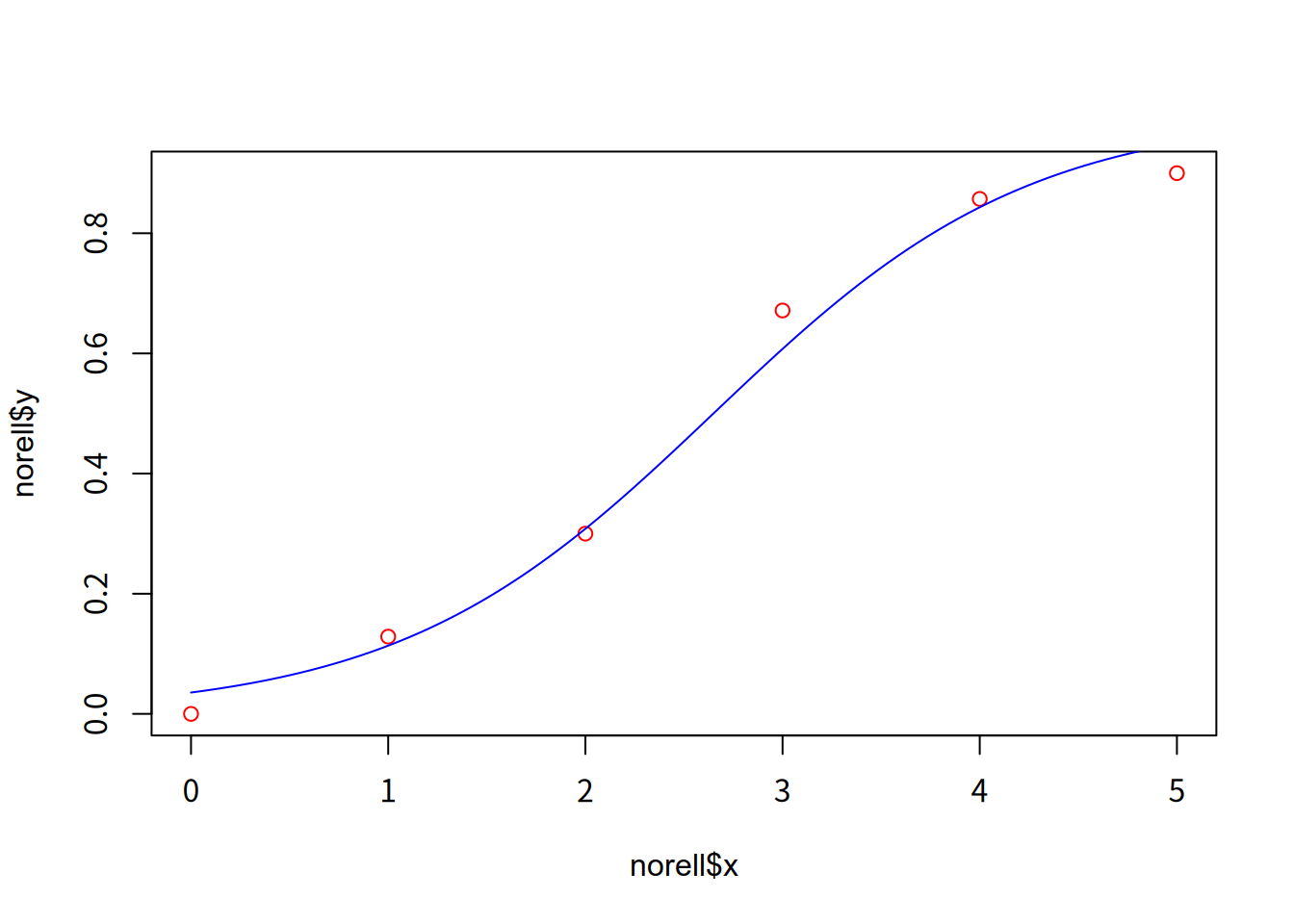
最后,画出响应比例与电流强度拟合的 logistic 回归曲线
norell$y = norell$success / norell$n
plot(norell$x, norell$y, col = "red")

d = seq(0, 5, len = 100)
p = predict(fit_logit, data.frame(x = d), type = "response")
lines(d, p, col = "blue")
下面是一个逻辑斯蒂回归实战案例,进一步学习该模型的应用。
第一步数据准备
数据为威斯康星大学的威廉.沃尔博格博士 1990 年发布的威斯康星州乳腺癌数据集。数据包含 699 个患者的组织样本,保存在 11 个变量的数据框中。
# 对原始数据添加变量名称
data(biopsy, package = "MASS")
names(biopsy) = c(
  "ID", "clumpThickness", "sizeUniformity", "shapeUniformity",
  "maginalAdhesion", "singleEpithelialCellSize", "bareNuclei",
  "blandChromatin", "normalNucleoli", "mitosis", "class"
)

biopsy |>
  subset(select = -ID) |>  # 去掉 ID 列,此列属于无关变量
  na.omit() -> data  # 缺失值占比很少,此处直接删除
- ID:样本ID号码
- clumpThickness:肿块厚度
- sizeUniformity:细胞大小的均匀性
- shapeUniformity:细胞形状的均匀性
- maginalAdhesion:边际附着力
- singleEpithelialCellSize:单个上皮细胞大小
- bareNuclei:裸核
- blandChromatin:乏味染色体
- normalNucleoli:正常核
- mitosis:有丝分裂
- class:类别。benign 表示良性,malignant 表示恶性。
第二步探索和理解数据
在分类问题中,我们可以通过作图来直观地理解数据。
library(tidyr)
library(ggplot2)
data |>
  pivot_longer(
    -class,
    names_to = "variable",
    values_to = "value"
  ) |>
  ggplot(aes(x = class, y = value)) +
  geom_boxplot() +
  facet_wrap(~ variable, ncol = 3)
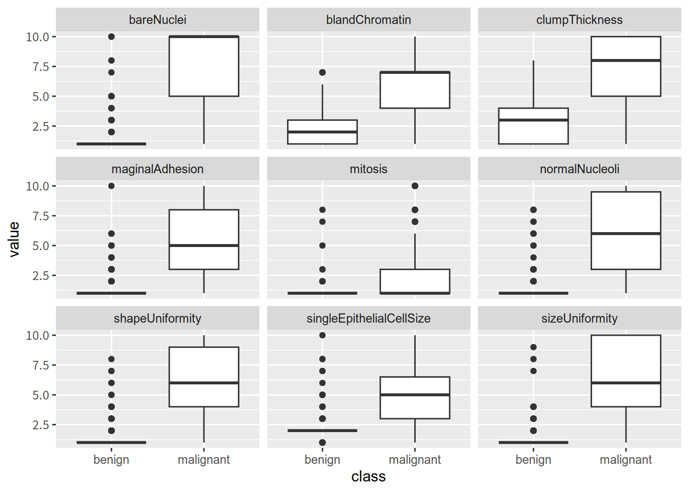
从上面的箱线图我们很难确定哪个特征在分类算法中是重要的,但是可以清楚地看到,除了有丝分裂(mitosis)特征变量外,几乎所有的特征变量关于良性和恶性两类细胞的中位数是有差异的。
逻辑斯蒂回归中的共线性也会使估计发生偏离,因此有必要检查特征变量之间的相关性。
library(corrplot)
bc = cor(data[, 1:9])
corrplot.mixed(bc)
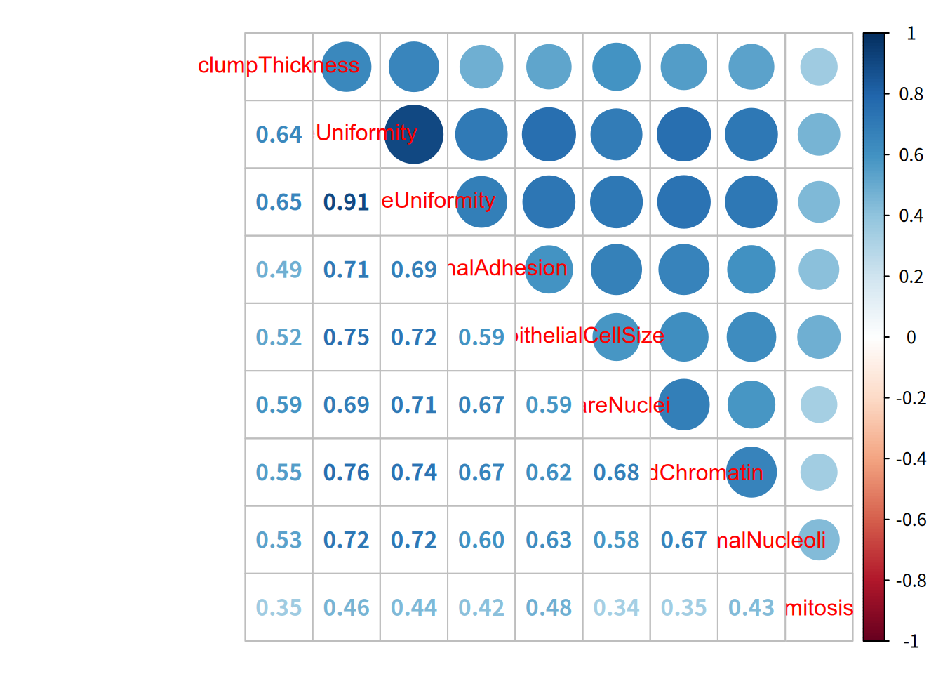
从相关系数可以看出,我们会遇到共线性问题,特笔试细胞大小均匀性和细胞形状的均匀性表现出非常明显的共线性。
第三步创建随机的训练和测试数据集
# 确定样本比例和样本量
split_size = 0.7
sample_size = floor(nrow(data) * split_size)

# 随机抽样产生训练数据和测试数据
set.seed(123)
train_ind = sample(nrow(data), size = sample_size)
train = data[train_ind, ]
test = data[-train_ind, ]
# ind = sample(
#   2, nrow(data),
#   replace = TRUE,
#   prob = c(sample_size, 1 - sample_size)
# )
# train = data[ind == 1, ]
# test = data[ind == 2, ]

# 确定特征变量和目标变量
label_train = train[, "class"]
data_train = subset(train, select = -class)

label_test = test[, "class"]
data_test = subset(test, select = -class)
第四步模型构建与评价
fit_logit = glm(class ~ ., family = binomial, data = train)
summary(fit_logit)
#>
#> Call:
#> glm(formula = class ~ ., family = binomial, data = train)
#>
#> Coefficients:
#>                          Estimate Std. Error z value Pr(>|z|)
#> (Intercept)              -9.50632    1.30102  -7.307 2.74e-13 ***
#> clumpThickness            0.36186    0.17133   2.112   0.0347 *
#> sizeUniformity            0.21625    0.26067   0.830   0.4068
#> shapeUniformity           0.21135    0.26471   0.798   0.4246
#> maginalAdhesion           0.33846    0.15098   2.242   0.0250 *
#> singleEpithelialCellSize  0.09755    0.22564   0.432   0.6655
#> bareNuclei                0.46052    0.11574   3.979 6.92e-05 ***
#> blandChromatin            0.44995    0.24127   1.865   0.0622 .
#> normalNucleoli            0.12504    0.13271   0.942   0.3461
#> mitosis                   0.49338    0.33330   1.480   0.1388
#> ---
#> Signif. codes:  0 '***' 0.001 '**' 0.01 '*' 0.05 '.' 0.1 ' ' 1
#>
#> (Dispersion parameter for binomial family taken to be 1)
#>
#>     Null deviance: 625.719  on 477  degrees of freedom
#> Residual deviance:  72.034  on 468  degrees of freedom
#> AIC: 92.034
#>
#> Number of Fisher Scoring iterations: 8
模型 95% 置信区间检验
confint(fit_logit)
#> Waiting for profiling to be done...
#>                                  2.5 %     97.5 %
#> (Intercept)              -1.251128e+01 -7.3071792
#> clumpThickness            4.318107e-02  0.7242080
#> sizeUniformity           -2.548373e-01  0.7839527
#> shapeUniformity          -3.387017e-01  0.7159371
#> maginalAdhesion           4.653941e-02  0.6576959
#> singleEpithelialCellSize -3.399246e-01  0.5427241
#> bareNuclei                2.467177e-01  0.7071627
#> blandChromatin           -8.285753e-04  0.9512558
#> normalNucleoli           -1.341275e-01  0.3963560
#> mitosis                  -3.326754e-02  1.1529143
回归系数转化为优势比
exp(coef(fit_logit))
#>              (Intercept)           clumpThickness           sizeUniformity
#>             7.438038e-05             1.436002e+00             1.241413e+00
#>          shapeUniformity          maginalAdhesion singleEpithelialCellSize
#>             1.235349e+00             1.402779e+00             1.102468e+00
#>               bareNuclei           blandChromatin           normalNucleoli
#>             1.584897e+00             1.568237e+00             1.133198e+00
#>                  mitosis
#>             1.637848e+00
如果系数大于1,就说明当特征的值增加时,优势比增加。反之,系数小于1,就说明当特征的值增加时,优势比减小。
通过变量筛选改进模型
fit_logit_new = step(fit_logit)
#> Start:  AIC=92.03
#> class ~ clumpThickness + sizeUniformity + shapeUniformity + maginalAdhesion +
#>     singleEpithelialCellSize + bareNuclei + blandChromatin +
#>     normalNucleoli + mitosis
#>
#>                            Df Deviance     AIC
#> - singleEpithelialCellSize  1   72.222  90.222
#> - shapeUniformity           1   72.641  90.641
#> - sizeUniformity            1   72.784  90.784
#> - normalNucleoli            1   72.933  90.933
#> <none>                          72.034  92.034
#> - mitosis                   1   75.303  93.303
#> - blandChromatin            1   75.861  93.861
#> - clumpThickness            1   77.037  95.037
#> - maginalAdhesion           1   77.179  95.179
#> - bareNuclei                1   91.113 109.113
#>
#> Step:  AIC=90.22
#> class ~ clumpThickness + sizeUniformity + shapeUniformity + maginalAdhesion +
#>     bareNuclei + blandChromatin + normalNucleoli + mitosis
#>
#>                   Df Deviance     AIC
#> - shapeUniformity  1   72.905  88.905
#> - sizeUniformity   1   73.203  89.203
#> - normalNucleoli   1   73.275  89.275
#> <none>                 72.222  90.222
#> - mitosis          1   75.509  91.509
#> - blandChromatin   1   76.415  92.415
#> - clumpThickness   1   77.063  93.063
#> - maginalAdhesion  1   78.586  94.586
#> - bareNuclei       1   93.771 109.771
#>
#> Step:  AIC=88.91
#> class ~ clumpThickness + sizeUniformity + maginalAdhesion + bareNuclei +
#>     blandChromatin + normalNucleoli + mitosis
#>
#>                   Df Deviance     AIC
#> - normalNucleoli   1   74.383  88.383
#> <none>                 72.905  88.905
#> - mitosis          1   76.009  90.009
#> - blandChromatin   1   77.107  91.107
#> - sizeUniformity   1   77.713  91.713
#> - clumpThickness   1   78.638  92.638
#> - maginalAdhesion  1   79.720  93.720
#> - bareNuclei       1   98.072 112.072
#>
#> Step:  AIC=88.38
#> class ~ clumpThickness + sizeUniformity + maginalAdhesion + bareNuclei +
#>     blandChromatin + mitosis
#>
#>                   Df Deviance     AIC
#> <none>                 74.383  88.383
#> - mitosis          1   77.102  89.102
#> - blandChromatin   1   80.092  92.092
#> - clumpThickness   1   81.012  93.012
#> - maginalAdhesion  1   82.090  94.090
#> - sizeUniformity   1   83.672  95.672
#> - bareNuclei       1  101.323 113.323
summary(fit_logit_new)
#>
#> Call:
#> glm(formula = class ~ clumpThickness + sizeUniformity + maginalAdhesion +
#>     bareNuclei + blandChromatin + mitosis, family = binomial,
#>     data = train)
#>
#> Coefficients:
#>                 Estimate Std. Error z value Pr(>|z|)
#> (Intercept)      -9.5415     1.2780  -7.466 8.26e-14 ***
#> clumpThickness    0.4051     0.1684   2.406  0.01612 *
#> sizeUniformity    0.4702     0.1768   2.660  0.00782 **
#> maginalAdhesion   0.3903     0.1456   2.680  0.00736 **
#> bareNuclei        0.4974     0.1112   4.472 7.73e-06 ***
#> blandChromatin    0.5318     0.2302   2.310  0.02088 *
#> mitosis           0.4634     0.3366   1.377  0.16858
#> ---
#> Signif. codes:  0 '***' 0.001 '**' 0.01 '*' 0.05 '.' 0.1 ' ' 1
#>
#> (Dispersion parameter for binomial family taken to be 1)
#>
#>     Null deviance: 625.719  on 477  degrees of freedom
#> Residual deviance:  74.383  on 471  degrees of freedom
#> AIC: 88.383
#>
#> Number of Fisher Scoring iterations: 8
模型对测试集数据进行分类
library(gmodels)
prob_test = predict(
  fit_logit_new,
  type = "response",
  newdata = data_test
)
CrossTable(
  x = label_test,
  y = ifelse(prob_test >= 0.5, "malignant", "benign"),
  dnn = c("Actual", "Predicted"),
  prop.chisq = FALSE
)
#>
#>
#>    Cell Contents
#> |-------------------------|
#> |                       N |
#> |           N / Row Total |
#> |           N / Col Total |
#> |         N / Table Total |
#> |-------------------------|
#>
#>
#> Total Observations in Table:  205
#>
#>
#>              | Predicted
#>       Actual |    benign | malignant | Row Total |
#> -------------|-----------|-----------|-----------|
#>       benign |       136 |         3 |       139 |
#>              |     0.978 |     0.022 |     0.678 |
#>              |     0.986 |     0.045 |           |
#>              |     0.663 |     0.015 |           |
#> -------------|-----------|-----------|-----------|
#>    malignant |         2 |        64 |        66 |
#>              |     0.030 |     0.970 |     0.322 |
#>              |     0.014 |     0.955 |           |
#>              |     0.010 |     0.312 |           |
#> -------------|-----------|-----------|-----------|
#> Column Total |       138 |        67 |       205 |
#>              |     0.673 |     0.327 |           |
#> -------------|-----------|-----------|-----------|
#>
#>
从预测结果看,预测的准确率是 (136 + 64) / 205 = 97.56%,效果令人满意。