
基于关联规则的购物篮分析
楚新元 / 2022-07-12
理解关联规则
购物篮分析主要用于超市数据。例如 {尿布,婴儿食品,啤酒} 在超市可能是一个典型的交易,该交易中识别的规则或许可以表示为如下形式 {尿布,婴儿食品}->{啤酒},换句话说,即“尿布和婴儿食品意味着啤酒”,这就是关联规则。
度量规则兴趣度
关联规则最广泛使用的方法就是 Apriori 算法。关联规则是否是令人感兴趣的取决于三个统计量:支持度、置信度、提升度。下面举例说明。
| 交易号 | 购买的商品 |
|---|---|
| 1 | {鲜花,慰问卡,苏打水} |
| 2 | {毛绒玩具熊,鲜花,气球,糖块} |
| 3 | {鲜花,慰问卡,糖块} |
| 4 | {毛绒玩具熊,气球,苏打水} |
| 5 | {鲜花,慰问卡,苏打水} |
支持度(support)。support(X) = count(X) / N,以上交易数据中,
{鲜花}的支持度为 4/5=0.8,{鲜花,慰问卡}的支持度为 3/5=0.6。鲜花和慰问卡同时购买的交易比数占整个交易比数的 60%;置信度(confidence)。confidence(X -> Y) = support(X, Y) / support(X),以上交易数据中
{鲜花}->{慰问卡}的置信度为 0.6/0.8 = 0.75。购买鲜花的所有交易中,有 75% 的交易还购买了慰问卡;提升度(lift)。lift(X->Y) = confidence(X->Y) / support(Y) = support(X, Y) / (support(X) * support(Y)),以上数据中
{鲜花}->{慰问卡}的提升度为 0.6/(0.8x0.6)=1.25。因为有 60% 的顾客购买了慰问卡,而购买鲜花的顾客有 75% 购买了慰问卡,所以提升度为 75/60=1.25;也可以理解为如果鲜花和慰问卡不想关的情况下同时购买的概率是 (0.8x0.6)=0.48,但是实际情况是两者同时购买的概率是 0.6,因此提升度为 0.6/0.48=1.25。
收集数据
数据改编自 R 中的 arules 包中的 Groceries 数据集,数据需要从 Packt 出版社网站下载 groceries.csv 文件。这里为了方便读者,可以直接从下面的链接下载数据。
library(arules)
groceries = read.transactions("./data/groceries.csv", sep = ",")
summary(groceries)
#> transactions as itemMatrix in sparse format with
#>  9835 rows (elements/itemsets/transactions) and
#>  169 columns (items) and a density of 0.02609146
#>
#> most frequent items:
#>       whole milk other vegetables       rolls/buns             soda
#>             2513             1903             1809             1715
#>           yogurt          (Other)
#>             1372            34055
#>
#> element (itemset/transaction) length distribution:
#> sizes
#>    1    2    3    4    5    6    7    8    9   10   11   12   13   14   15   16
#> 2159 1643 1299 1005  855  645  545  438  350  246  182  117   78   77   55   46
#>   17   18   19   20   21   22   23   24   26   27   28   29   32
#>   29   14   14    9   11    4    6    1    1    1    1    3    1
#>
#>    Min. 1st Qu.  Median    Mean 3rd Qu.    Max.
#>   1.000   2.000   3.000   4.409   6.000  32.000
#>
#> includes extended item information - examples:
#>             labels
#> 1 abrasive cleaner
#> 2 artif. sweetener
#> 3   baby cosmetics
原始数据的前 5 行如下所示:
citrus fruit,semi-finished bread,margarine,ready soups
tropical fruit,yogurt,coffee
whole milk
pip fruit,yogurt,cream cheese,meat spreads
other vegetables,whole milk,condensed milk,long life bakery product
注:arules 包中的 read.transactions 可以产生一个稀疏矩阵,read.csv 函数则不能。
输出信息中的第一块提供了系数矩阵概要,9835 行表示交易次数,169 列指的是购物篮中的 169 类不同的商品。如果在相应的交易中该商品被购买了,则矩阵中该单元格为 1,否则为 0。密度值为 0.02609146 指的是矩阵中非零单元的比例。所以可以计算出该超市 30 天内共有 9835x169x0.02609146=43367 件商品被购买(忽略同样的商品可能被重复购买的事实)。进一步,我们可以确定平均交易包含了 43367/9835=4.409 种不同的商品。
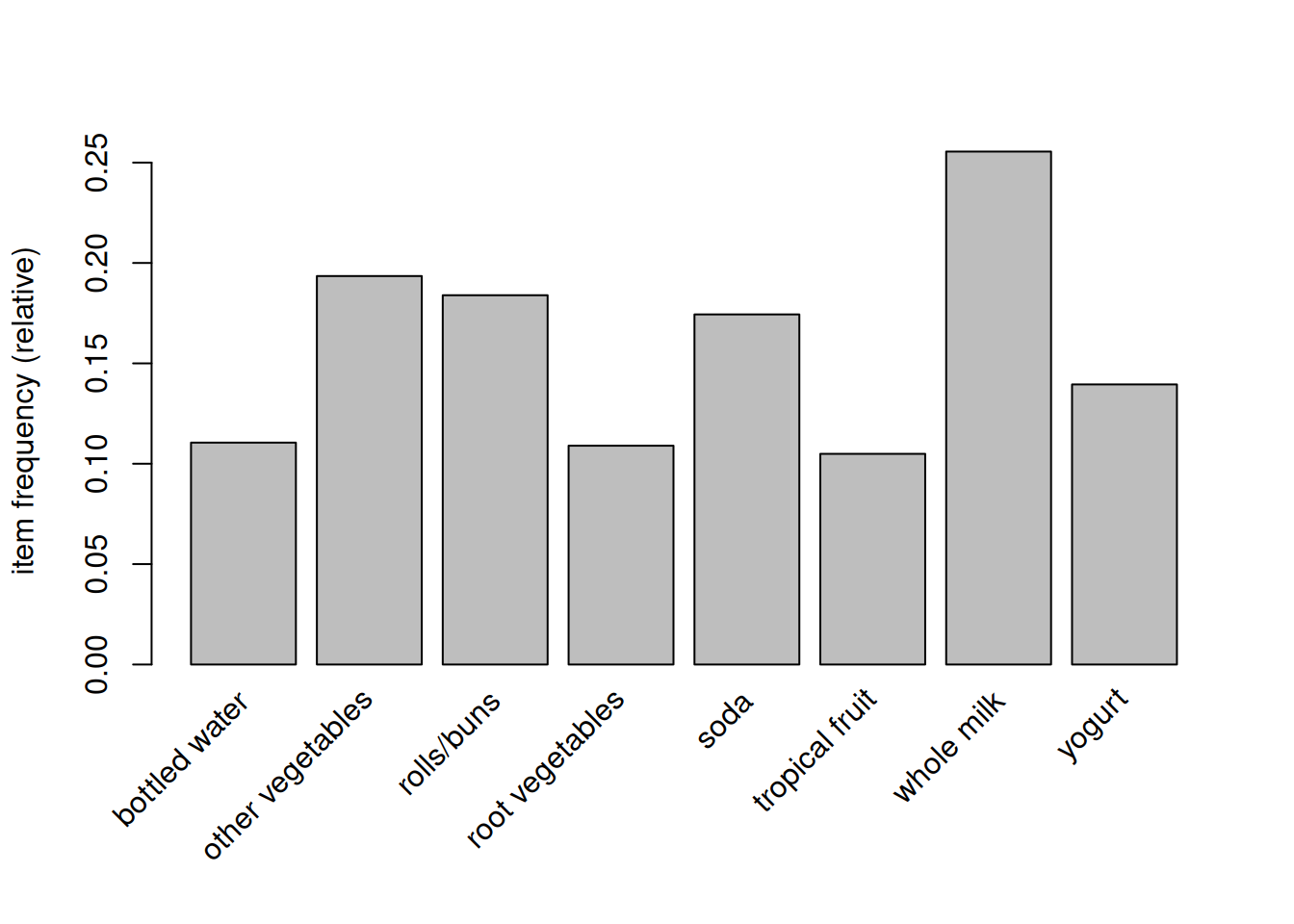
输出信息第二块我们可以看到 whole milk(全脂牛奶)出现的概率为 2513/9835x100%=25.6%。
输出信息第三块呈现了一组关于交易规模的统计。总共有 2159 次交易只包含一件单一商品。而有一次交易包含了 32 类商品。
系数矩阵前三件商品(系数矩阵中商品所在的列按字母表顺序排序)的支持度为
itemFrequency(groceries[, 1:3])
#> abrasive cleaner artif. sweetener   baby cosmetics
#>     0.0035587189     0.0032536858     0.0006100661
可视化商品的支持度
itemFrequencyPlot(groceries, support = 0.1) # 支持度为 10% 的商品
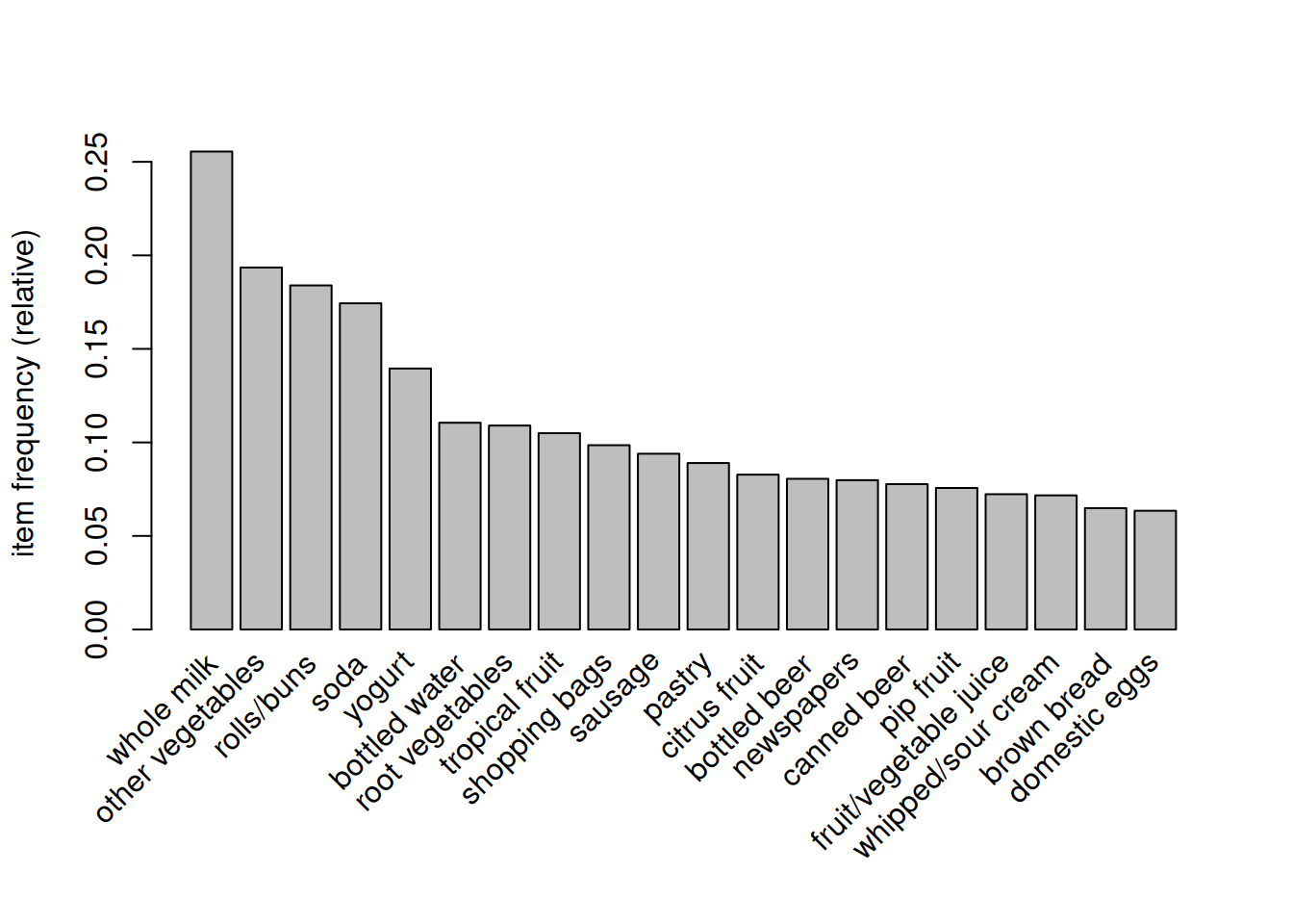
itemFrequencyPlot(groceries, topN = 20) # 支持度前 20 的商品
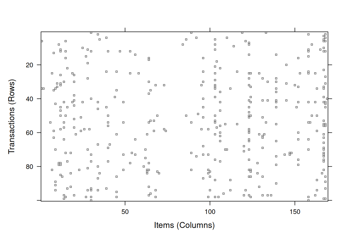
image(groceries[1:100, ]) # 前 100 次交易系数矩阵。结果是 100 行 169 列矩阵图。
基于数据训练模型
groceries_rules = apriori(
  groceries,
  parameter = list(
    support = 0.006,
    confidence = 0.25,
    minlen = 2   # 消除少于两类商品的规则
  )
)
#> Apriori
#>
#> Parameter specification:
#>  confidence minval smax arem  aval originalSupport maxtime support minlen
#>        0.25    0.1    1 none FALSE            TRUE       5   0.006      2
#>  maxlen target  ext
#>      10  rules TRUE
#>
#> Algorithmic control:
#>  filter tree heap memopt load sort verbose
#>     0.1 TRUE TRUE  FALSE TRUE    2    TRUE
#>
#> Absolute minimum support count: 59
#>
#> set item appearances ...[0 item(s)] done [0.00s].
#> set transactions ...[169 item(s), 9835 transaction(s)] done [0.00s].
#> sorting and recoding items ... [109 item(s)] done [0.00s].
#> creating transaction tree ... done [0.00s].
#> checking subsets of size 1 2 3 4 done [0.00s].
#> writing ... [463 rule(s)] done [0.00s].
#> creating S4 object  ... done [0.00s].
groceries_rules
#> set of 463 rules
groceries_rules 对象包含了 463 个关联规则,为了确定它们对我们是否有用,我们必须深入挖掘。(注:上述的参数可以根据需要调整。)
模型评价与应用
summary(groceries_rules)
#> set of 463 rules
#>
#> rule length distribution (lhs + rhs):sizes
#>   2   3   4
#> 150 297  16
#>
#>    Min. 1st Qu.  Median    Mean 3rd Qu.    Max.
#>   2.000   2.000   3.000   2.711   3.000   4.000
#>
#> summary of quality measures:
#>     support           confidence        coverage             lift
#>  Min.   :0.006101   Min.   :0.2500   Min.   :0.009964   Min.   :0.9932
#>  1st Qu.:0.007117   1st Qu.:0.2971   1st Qu.:0.018709   1st Qu.:1.6229
#>  Median :0.008744   Median :0.3554   Median :0.024809   Median :1.9332
#>  Mean   :0.011539   Mean   :0.3786   Mean   :0.032608   Mean   :2.0351
#>  3rd Qu.:0.012303   3rd Qu.:0.4495   3rd Qu.:0.035892   3rd Qu.:2.3565
#>  Max.   :0.074835   Max.   :0.6600   Max.   :0.255516   Max.   :3.9565
#>      count
#>  Min.   : 60.0
#>  1st Qu.: 70.0
#>  Median : 86.0
#>  Mean   :113.5
#>  3rd Qu.:121.0
#>  Max.   :736.0
#>
#> mining info:
#>       data ntransactions support confidence
#>  groceries          9835   0.006       0.25
#>                                                                                         call
#>  apriori(data = groceries, parameter = list(support = 0.006, confidence = 0.25, minlen = 2))
在我们的规则集中,有 150 个规则只包含 2 类商品,297 个规则包含 3 类商品,16 个规则包含 4 类商品。我们可以用 inspect() 函数看一看具体规则。
inspect(groceries_rules[1:3, ])
#>     lhs                rhs               support     confidence coverage
#> [1] {potted plants} => {whole milk}      0.006914082 0.4000000  0.01728521
#> [2] {pasta}         => {whole milk}      0.006100661 0.4054054  0.01504830
#> [3] {herbs}         => {root vegetables} 0.007015760 0.4312500  0.01626843
#>     lift     count
#> [1] 1.565460 68
#> [2] 1.586614 60
#> [3] 3.956477 69
对于第一条规则,我们发现 potted plantsh 和 whole milk 同时购买的交易比数占整个交易比数的 0.6914%;购买 potted plantsh 的所有交易中,有 40% 的交易还购买了 whole milk;提升度(lift)值告诉我们假定一个顾客购买了 potted plantsh,他相对于一般顾客购买 whole milk 的有多大倾向程度。因为我们知道大约有 25.6% 的顾客购买了 whole milk,而购买 potted plantsh 的顾客有 40% 购买了 whole milk,所以我们可以计算提升度为 40/25.6=1.56。
我们可以利用sort()函数,根据规则的支持度(support)、置信度(confidence)或者提升度(lift)进行排序。这里以提升度举例说明。
inspect(sort(groceries_rules, by = "lift")[1:5, ])
#>     lhs                    rhs                      support confidence   coverage     lift count
#> [1] {herbs}             => {root vegetables}    0.007015760  0.4312500 0.01626843 3.956477    69
#> [2] {berries}           => {whipped/sour cream} 0.009049314  0.2721713 0.03324860 3.796886    89
#> [3] {other vegetables,
#>      tropical fruit,
#>      whole milk}        => {root vegetables}    0.007015760  0.4107143 0.01708185 3.768074    69
#> [4] {beef,
#>      other vegetables}  => {root vegetables}    0.007930859  0.4020619 0.01972547 3.688692    78
#> [5] {other vegetables,
#>      tropical fruit}    => {pip fruit}          0.009456024  0.2634561 0.03589222 3.482649    93
这些规则似乎比我们之前看到的更令人感兴趣。因为提升度很高,关联关系密切。
我们还可以针对我们感兴趣的项目单独提取出来进行分析,比如营销团队可能对 berries 感兴趣,我们可以提取出那些规则中包含 berries 的所有规则。
inspect(subset(groceries_rules, items %in% "berries"))
#>     lhs          rhs                  support     confidence coverage  lift
#> [1] {berries} => {whipped/sour cream} 0.009049314 0.2721713  0.0332486 3.796886
#> [2] {berries} => {yogurt}             0.010574479 0.3180428  0.0332486 2.279848
#> [3] {berries} => {other vegetables}   0.010269446 0.3088685  0.0332486 1.596280
#> [4] {berries} => {whole milk}         0.011794611 0.3547401  0.0332486 1.388328
#>     count
#> [1]  89
#> [2] 104
#> [3] 101
#> [4] 116
将关联规则保存到数据框
groceries_rules_df = as(groceries_rules, "data.frame")
head(groceries_rules_df)
#>                                rules     support confidence   coverage     lift
#> 1    {potted plants} => {whole milk} 0.006914082  0.4000000 0.01728521 1.565460
#> 2            {pasta} => {whole milk} 0.006100661  0.4054054 0.01504830 1.586614
#> 3       {herbs} => {root vegetables} 0.007015760  0.4312500 0.01626843 3.956477
#> 4      {herbs} => {other vegetables} 0.007727504  0.4750000 0.01626843 2.454874
#> 5            {herbs} => {whole milk} 0.007727504  0.4750000 0.01626843 1.858983
#> 6 {processed cheese} => {whole milk} 0.007015760  0.4233129 0.01657346 1.656698
#>   count
#> 1    68
#> 2    60
#> 3    69
#> 4    76
#> 5    76
#> 6    69