
自相关:诊断与处理
楚新元 / 2021-09-05
如果对于不同的样本点,随机误差项之间不再是不相关的,而是存在某种相关性,则认为出现了序列相关性。 古扎拉蒂《经济计量学精要》表 10-7 给出的1980 ~ 2006年间股票价格和 GDP 的数据。
载入数据
options(digits = 4)
library(readxl)
library(dplyr)
library(kableExtra)
data = read_xls(
  "data/Table10_7.xls",
  skip = 4, n_max = 27
)[, 2:3]
data %>%
  kable() %>%
   kable_styling(
     bootstrap_options = "striped",
     font_size = 14
  )
| NYSE | GDP |
|---|---|
| 720.1 | 2790 |
| 782.6 | 3128 |
| 728.8 | 3255 |
| 979.5 | 3537 |
| 977.3 | 3933 |
| 1143.0 | 4220 |
| 1438.0 | 4463 |
| 1709.8 | 4740 |
| 1585.1 | 5104 |
| 1903.4 | 5484 |
| 1939.5 | 5803 |
| 2181.7 | 5996 |
| 2421.5 | 6338 |
| 2639.0 | 6657 |
| 2687.0 | 7072 |
| 3078.6 | 7398 |
| 3787.2 | 7817 |
| 4827.4 | 8304 |
| 5818.3 | 8747 |
| 6546.8 | 9268 |
| 6805.9 | 9817 |
| 6397.9 | 10128 |
| 5578.9 | 10470 |
| 5447.5 | 10961 |
| 6612.6 | 11686 |
| 7349.0 | 12434 |
| 8358.0 | 13195 |
建立一元线性回归模型
model = lm(NYSE ~ GDP, data = data)
summary(model)
#>
#> Call:
#> lm(formula = NYSE ~ GDP, data = data)
#>
#> Residuals:
#>    Min     1Q Median     3Q    Max
#>  -1002   -446   -101    323   1404
#>
#> Coefficients:
#>              Estimate Std. Error t value Pr(>|t|)
#> (Intercept) -2.02e+03   3.06e+02   -6.58  6.8e-07 ***
#> GDP          7.72e-01   3.96e-02   19.52  < 2e-16 ***
#> ---
#> Signif. codes:  0 '***' 0.001 '**' 0.01 '*' 0.05 '.' 0.1 ' ' 1
#>
#> Residual standard error: 615 on 25 degrees of freedom
#> Multiple R-squared:  0.938,	Adjusted R-squared:  0.936
#> F-statistic:  381 on 1 and 25 DF,  p-value: <2e-16
自相关的诊断
观察残差走势
# plot(model, which = 1)
plot(model$residuals)
abline(h = 0, lty = 3)
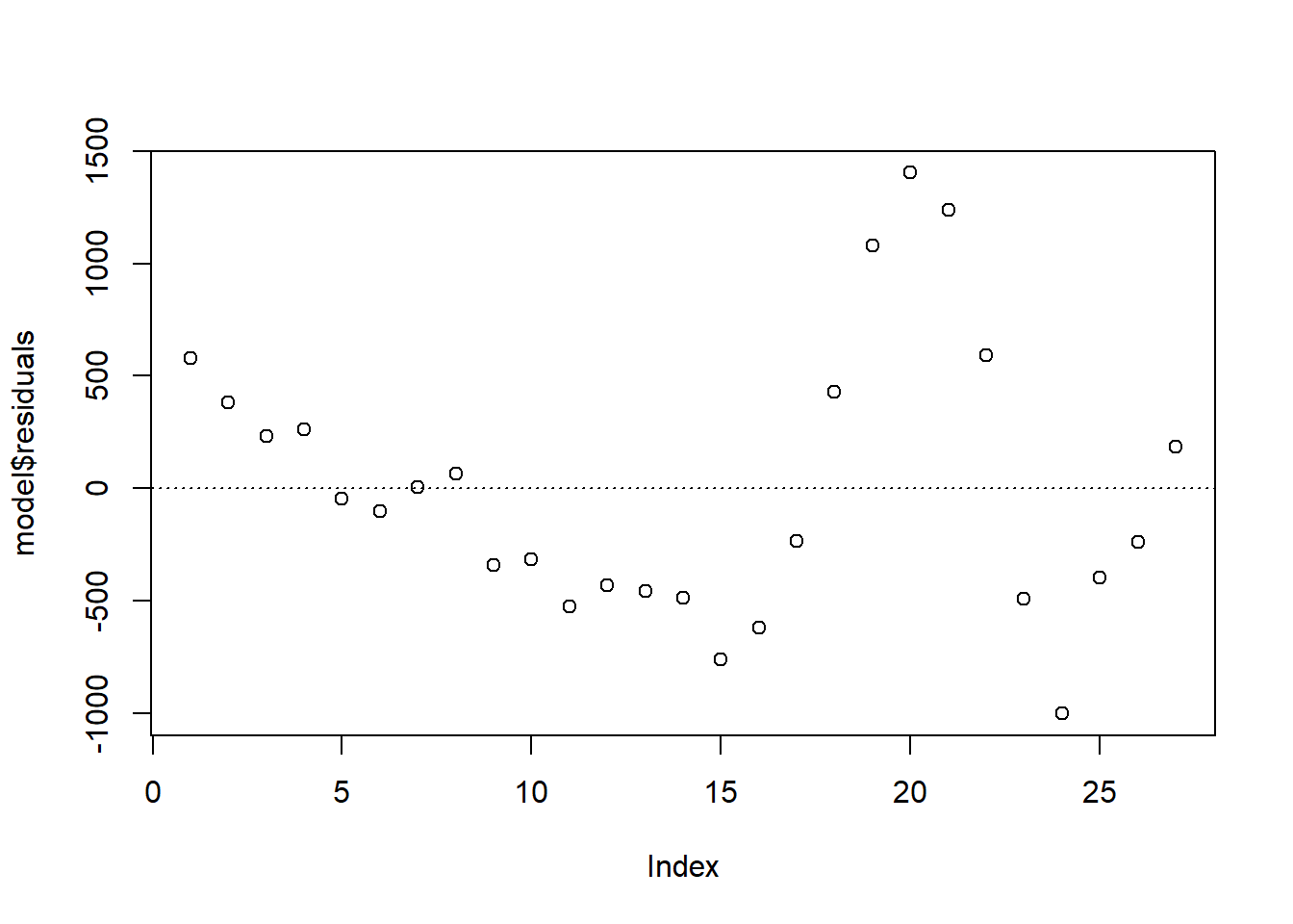
从图中可以看出,残差呈现出有规律的波动,初步判断模型存在自相关。
观察残差和残差滞后一阶的散点图
e = model$residuals
plot(e[-1] ~ e[-nrow(data)], xlab = "e(-1)", ylab = "e")
abline(h = 0, lty = 3)
abline(v = 0, lty = 3)
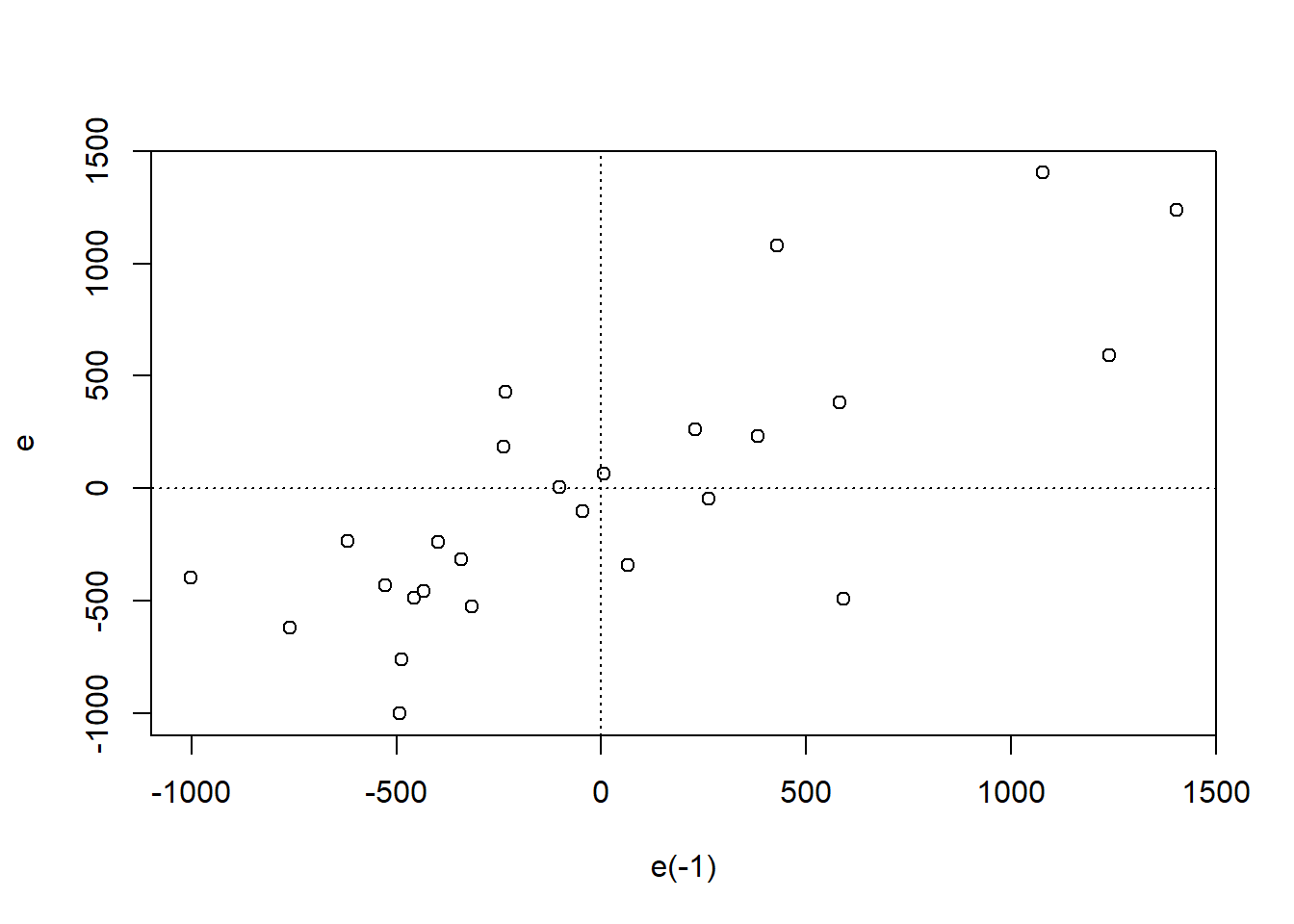
残差滞后一阶和残差散点图上,散点主要分布在一、三象限,初步判断模型存在正自相关。
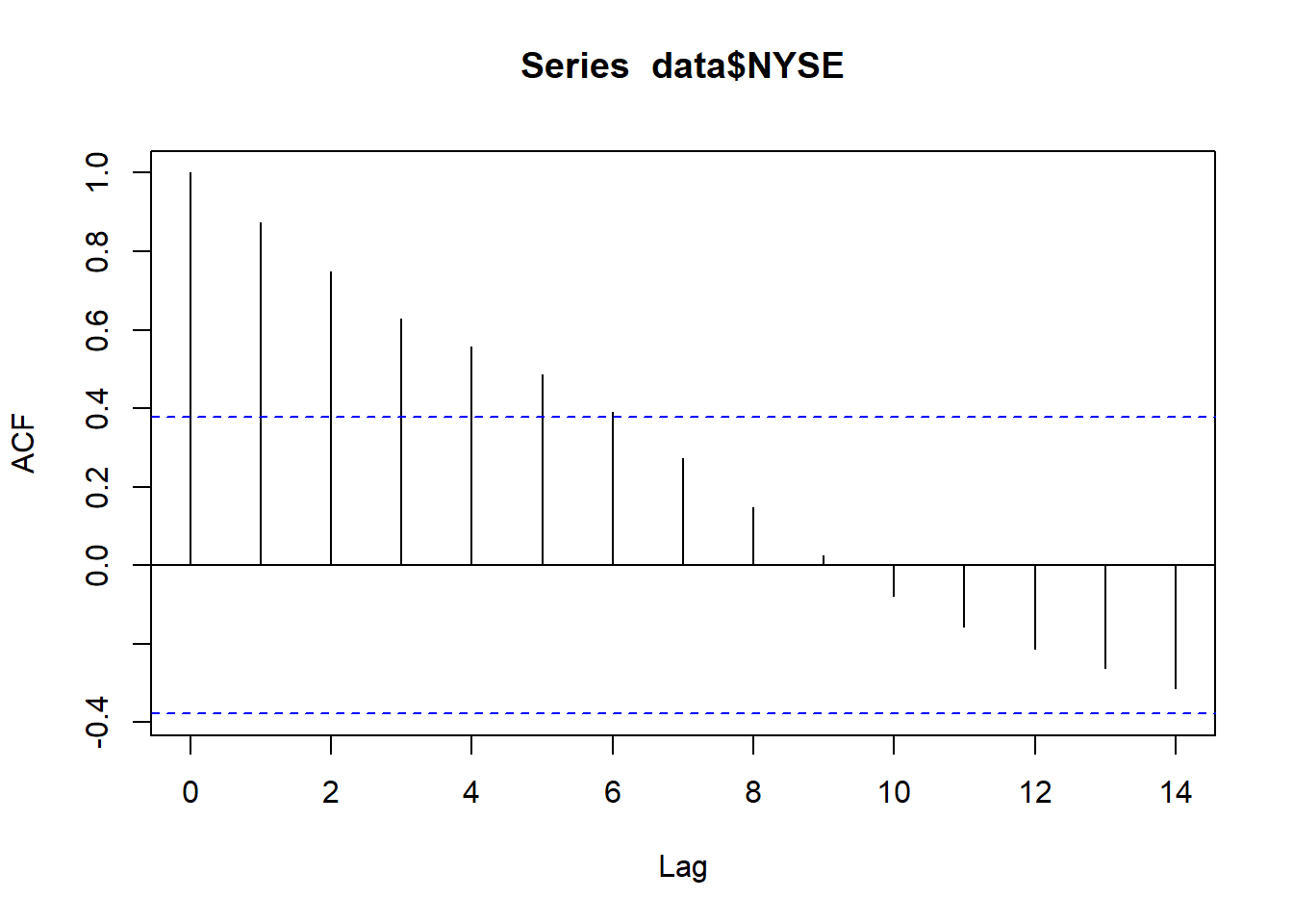
自相关图
acf(data$NYSE)
DW 一阶自相关检验
library(lmtest)
dwtest(model)
#>
#> 	Durbin-Watson test
#>
#> data:  model
#> DW = 0.43, p-value = 2e-08
#> alternative hypothesis: true autocorrelation is greater than 0
当 n = 27, k’ = 1时,显著性水平为 5% 的 DW 统计量临界值为 1.316 和 1.469。 因为 DW 统计量的值为 0.4285,小于 1.316,因此模型存在正一阶自相关。
LM 检验
bgtest(model)
#>
#> 	Breusch-Godfrey test for serial correlation of order up to 1
#>
#> data:  model
#> LM test = 16, df = 1, p-value = 7e-05
LM 检验拒绝无自相关原假设,表明模型存在自相关。
\(\rho\) 值通过 DW 值估计得到,用 OLS 估计广义差分方程
根据 DW 值计算 \(\rho\) 值
ρ_hat_dw = 1 - dwtest(model)$statistic / 2
names(ρ_hat_dw) = "ρ_hat_dw"
print(ρ_hat_dw)
#> ρ_hat_dw
#>    0.7858
估计原模型的 \(\beta_{1}\) 和 \(\beta_{2}\) (舍去第一个观测值)
data %>%
  mutate(
    NYSE_star = NYSE - ρ_hat_dw * lag(NYSE, 1),  # 此处lag是滞后的意思
    GDP_star = GDP - ρ_hat_dw * lag(GDP, 1)
  ) %>%
  na.omit() %>%
  lm(NYSE_star ~ GDP_star, data = .) -> model_star_lack
  # 此处差分损失一个样本。
  # 如果样本量足够多,可以不用补齐第一个缺失值。
  # 如果样本量小,可以通过sqrt(1-ρ^2)*Y[1]、sqrt(1-ρ^2)*X[1]补齐。

beta1_lack = coef(model_star_lack)[1] / (1 - ρ_hat_dw)
beta2_lack = coef(model_star_lack)[2]
names(beta2_lack) = "GDP"

summary(model_star_lack)
#>
#> Call:
#> lm(formula = NYSE_star ~ GDP_star, data = .)
#>
#> Residuals:
#>    Min     1Q Median     3Q    Max
#> -996.2 -150.5   22.8  177.6  727.0
#>
#> Coefficients:
#>             Estimate Std. Error t value Pr(>|t|)
#> (Intercept) -617.954    205.309   -3.01   0.0061 **
#> GDP_star       0.862      0.102    8.47  1.1e-08 ***
#> ---
#> Signif. codes:  0 '***' 0.001 '**' 0.01 '*' 0.05 '.' 0.1 ' ' 1
#>
#> Residual standard error: 378 on 24 degrees of freedom
#> Multiple R-squared:  0.749,	Adjusted R-squared:  0.739
#> F-statistic: 71.7 on 1 and 24 DF,  p-value: 1.14e-08

# 利用 DW-test 对 model_star_lack 模型进行检验
dwtest(model_star_lack)
#>
#> 	Durbin-Watson test
#>
#> data:  model_star_lack
#> DW = 0.91, p-value = 5e-04
#> alternative hypothesis: true autocorrelation is greater than 0

# 利用 LM-test 对 model_star_lack 模型进行检验
bgtest(model_star_lack)
#>
#> 	Breusch-Godfrey test for serial correlation of order up to 1
#>
#> data:  model_star_lack
#> LM test = 7.6, df = 1, p-value = 0.006
还原后的估计方程: $$ \widehat{NYSE} = -2884.2875 + 0.8624 * GDP $$
估计原模型的 \(\beta_{1}\) 和 \(\beta_{2}\) (包含第一个观测值)
data %>%
  mutate(
    NYSE_star = NYSE - ρ_hat_dw * lag(NYSE, 1),
    GDP_star = GDP - ρ_hat_dw * lag(GDP, 1),
    NYSE_star_1 = sqrt(1-ρ_hat_dw^2) * NYSE * c(1,rep(0,nrow(data)-1)),
    GDP_star_1 = sqrt(1-ρ_hat_dw^2) * GDP * c(1,rep(0,nrow(data)-1))
  ) -> data_NA

data_NA$NYSE_star[is.na(data_NA$NYSE_star)] = 0
data_NA$GDP_star[is.na(data_NA$GDP_star)] = 0

data_NA %>%
  mutate(
    NYSE_star_full = NYSE_star + NYSE_star_1,
    GDP_star_full = GDP_star + GDP_star_1
  ) %>%
  lm(
    NYSE_star_full ~ GDP_star_full,
    data = .
  ) -> model_star_full

beta1_full = coef(model_star_full)[1] / (1 - ρ_hat_dw)
beta2_full = coef(model_star_full)[2]
names(beta2_full) = "GDP"

summary(model_star_full)
#>
#> Call:
#> lm(formula = NYSE_star_full ~ GDP_star_full, data = .)
#>
#> Residuals:
#>    Min     1Q Median     3Q    Max
#> -983.4 -179.8   37.8  194.1  741.1
#>
#> Coefficients:
#>               Estimate Std. Error t value Pr(>|t|)
#> (Intercept)   -642.233    204.978   -3.13   0.0044 **
#> GDP_star_full    0.867      0.102    8.48  7.9e-09 ***
#> ---
#> Signif. codes:  0 '***' 0.001 '**' 0.01 '*' 0.05 '.' 0.1 ' ' 1
#>
#> Residual standard error: 380 on 25 degrees of freedom
#> Multiple R-squared:  0.742,	Adjusted R-squared:  0.732
#> F-statistic:   72 on 1 and 25 DF,  p-value: 7.91e-09

# 利用 DW-test 对 model_star_full 模型进行检验
dwtest(model_star_full)
#>
#> 	Durbin-Watson test
#>
#> data:  model_star_full
#> DW = 0.92, p-value = 5e-04
#> alternative hypothesis: true autocorrelation is greater than 0

# 利用 LM-test 对 model_star_full 模型进行检验
bgtest(model_star_full)
#>
#> 	Breusch-Godfrey test for serial correlation of order up to 1
#>
#> data:  model_star_full
#> LM test = 7, df = 1, p-value = 0.008
还原后的估计方程: $$ \widehat{NYSE} = -2997.6114 + 0.867 * GDP $$
\(\rho\) 值通过 OLS 残差估计得到
根据 OLS 残差估计 \(\rho\) 值
uxfit = lm(
  model$residuals ~ 0 + lag(model$residuals),
  data = data
)
ρ_hat_ols = coef(uxfit)[1]
names(ρ_hat_ols) = "ρ_hat_ols"
print(ρ_hat_ols)
#> ρ_hat_ols
#>     0.7689
估计原模型的 \(\beta_{1}\) 和 \(\beta_{2}\) (舍去第一个观测值)
data %>%
  mutate(
    NYSE_star = NYSE - ρ_hat_ols * lag(NYSE, 1),
    GDP_star = GDP - ρ_hat_ols * lag(GDP, 1)
  ) %>%
  na.omit() %>%
  lm(
    NYSE_star ~ GDP_star,
    data = .
  ) -> model_star_lack2
  # 此处差分损失一个样本。
  # 如果样本量足够多,可以不用补齐第一个缺失值。
  # 如果样本量小,可以通过sqrt(1-ρ^2)*Y[1]、sqrt(1-ρ^2)*X[1]补齐。

beta1_lack2 = coef(model_star_lack2)[1] / (1 - ρ_hat_ols)
beta2_lack2 = coef(model_star_lack2)[2]
names(beta2_lack2) = "GDP"

summary(model_star_lack2)
#>
#> Call:
#> lm(formula = NYSE_star ~ GDP_star, data = .)
#>
#> Residuals:
#>    Min     1Q Median     3Q    Max
#> -985.7 -149.8   21.5  178.3  735.0
#>
#> Coefficients:
#>              Estimate Std. Error t value Pr(>|t|)
#> (Intercept) -647.2103   205.0171   -3.16   0.0043 **
#> GDP_star       0.8547     0.0957    8.93  4.3e-09 ***
#> ---
#> Signif. codes:  0 '***' 0.001 '**' 0.01 '*' 0.05 '.' 0.1 ' ' 1
#>
#> Residual standard error: 379 on 24 degrees of freedom
#> Multiple R-squared:  0.769,	Adjusted R-squared:  0.759
#> F-statistic: 79.7 on 1 and 24 DF,  p-value: 4.29e-09

# 利用 DW-test 对 model_star_lack2 模型进行检验
dwtest(model_star_lack2)
#>
#> 	Durbin-Watson test
#>
#> data:  model_star_lack2
#> DW = 0.9, p-value = 4e-04
#> alternative hypothesis: true autocorrelation is greater than 0

# 利用 LM-test 对 model_star_lack2 模型进行检验
bgtest(model_star_lack2)
#>
#> 	Breusch-Godfrey test for serial correlation of order up to 1
#>
#> data:  model_star_lack2
#> LM test = 7.8, df = 1, p-value = 0.005
还原后的估计方程: $$ \widehat{NYSE} = -2800.1965 + 0.8547 * GDP $$
估计原模型的 \(\beta_{1}\) 和 \(\beta_{2}\) (包含第一个观测值)
data %>%
  mutate(
    NYSE_star = NYSE - ρ_hat_ols * lag(NYSE, 1),
    GDP_star = GDP - ρ_hat_ols * lag(GDP, 1),
    NYSE_star_1 = sqrt(1-ρ_hat_ols^2) * NYSE * c(1,rep(0,nrow(data)-1)),
    GDP_star_1 = sqrt(1-ρ_hat_ols^2) * GDP * c(1,rep(0,nrow(data)-1))
  ) -> data_NA2

data_NA2$NYSE_star[is.na(data_NA2$NYSE_star)] = 0
data_NA2$GDP_star[is.na(data_NA2$GDP_star)] = 0

data_NA2 %>%
  mutate(
    NYSE_star_full = NYSE_star + NYSE_star_1,
    GDP_star_full = GDP_star + GDP_star_1
  ) %>%
  lm(
    NYSE_star_full ~ GDP_star_full,
    data = .
  ) -> model_star_full2

b1_full2 = coef(model_star_full2)[1] / (1 - ρ_hat_ols)
b2_full2 = coef(model_star_full2)[2]
names(b2_full2) = "GDP"

summary(model_star_full2)
#>
#> Call:
#> lm(formula = NYSE_star_full ~ GDP_star_full, data = .)
#>
#> Residuals:
#>    Min     1Q Median     3Q    Max
#> -974.1 -180.7   36.1  194.2  748.4
#>
#> Coefficients:
#>                Estimate Std. Error t value Pr(>|t|)
#> (Intercept)   -673.4730   204.2343   -3.30   0.0029 **
#> GDP_star_full    0.8601     0.0959    8.97  2.8e-09 ***
#> ---
#> Signif. codes:  0 '***' 0.001 '**' 0.01 '*' 0.05 '.' 0.1 ' ' 1
#>
#> Residual standard error: 380 on 25 degrees of freedom
#> Multiple R-squared:  0.763,	Adjusted R-squared:  0.753
#> F-statistic: 80.4 on 1 and 25 DF,  p-value: 2.75e-09

# 利用 DW-test 对 model_star_full2 模型进行检验
dwtest(model_star_full2)
#>
#> 	Durbin-Watson test
#>
#> data:  model_star_full2
#> DW = 0.92, p-value = 4e-04
#> alternative hypothesis: true autocorrelation is greater than 0

# 利用 LM-test 对 model_star_full2 模型进行检验
bgtest(model_star_full2)
#>
#> 	Breusch-Godfrey test for serial correlation of order up to 1
#>
#> data:  model_star_full2
#> LM test = 7.2, df = 1, p-value = 0.007
还原后的估计方程: $$ \widehat{NYSE} = -2913.8235 + 0.8601 * GDP $$
利用一阶差分法对变换后的模型进行估计
data %>%
  mutate(
    NYSE_star = NYSE - lag(NYSE, 1),
    GDP_star = GDP - lag(GDP, 1)
  ) %>%
  na.omit() %>%
  lm(
    NYSE_star ~ 0 + GDP_star,
    data = .
  ) -> model_star_3

beta2_3 = coef(model_star_3)
names(beta2_3) = "GDP"
beta1_3 = mean(data$NYSE) - beta2_3 * mean(data$GDP)
names(beta1_3 ) = "Intercept"

summary(model_star_3)
#>
#> Call:
#> lm(formula = NYSE_star ~ 0 + GDP_star, data = .)
#>
#> Residuals:
#>     Min      1Q  Median      3Q     Max
#> -1115.6  -238.5   -34.7   103.3   616.9
#>
#> Coefficients:
#>          Estimate Std. Error t value Pr(>|t|)
#> GDP_star    0.868      0.183    4.75  7.1e-05 ***
#> ---
#> Signif. codes:  0 '***' 0.001 '**' 0.01 '*' 0.05 '.' 0.1 ' ' 1
#>
#> Residual standard error: 401 on 25 degrees of freedom
#> Multiple R-squared:  0.474,	Adjusted R-squared:  0.453
#> F-statistic: 22.6 on 1 and 25 DF,  p-value: 7.14e-05

# 利用 LM-test 对 model_star_3 模型进行检验
bgtest(model_star_3)
#>
#> 	Breusch-Godfrey test for serial correlation of order up to 1
#>
#> data:  model_star_3
#> LM test = 7.1, df = 1, p-value = 0.008
还原后的估计方程: $$ \widehat{NYSE} = -2701.4792 + 0.8684 * GDP $$